Table of Contents
Master method
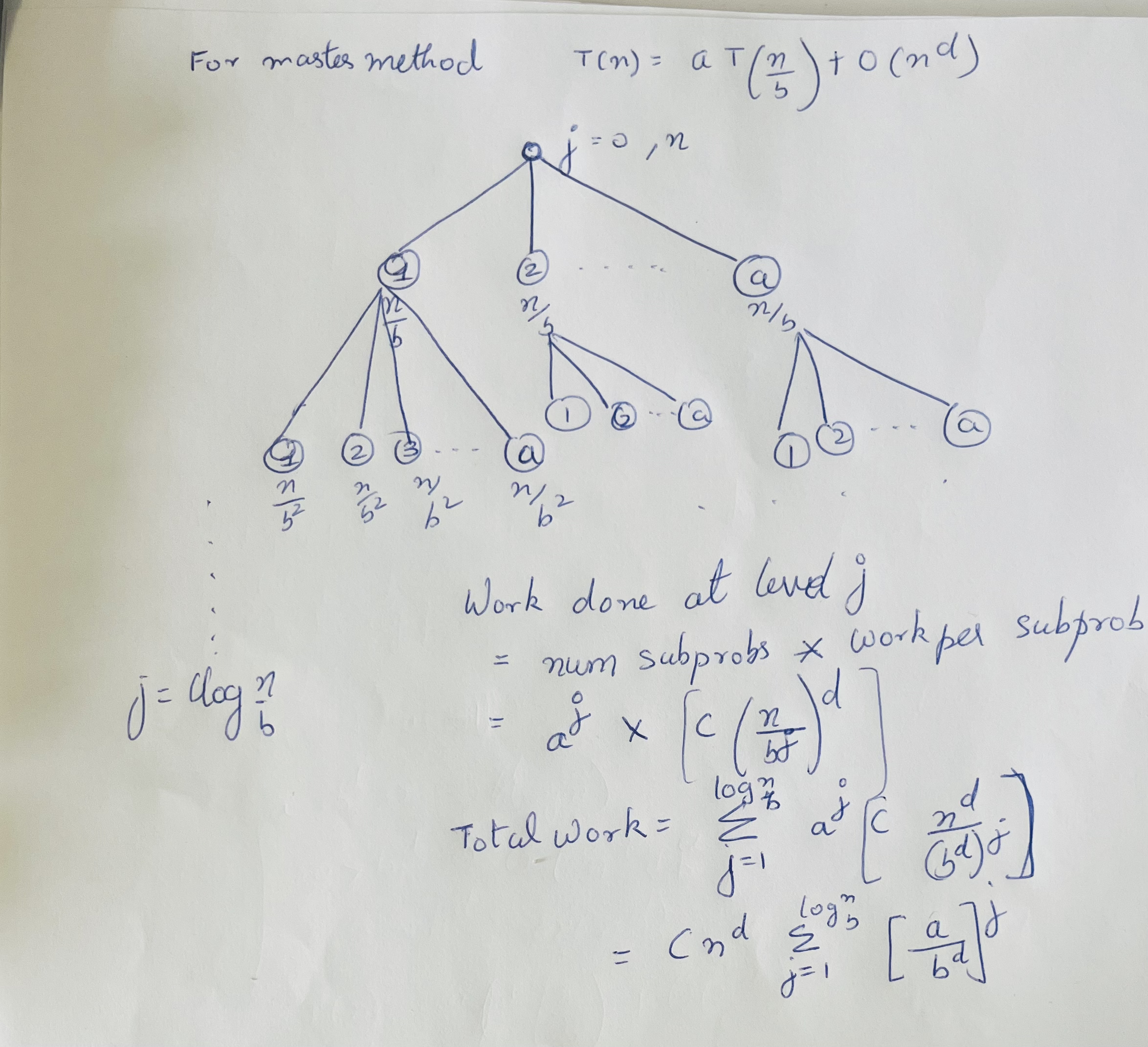
Master method describes the time complexity of recursive divide and conquer algorithms. Assumes that each subproblem of the recursion is of the same size. Here \(a\) is the number of subproblems, \(\dfrac{n}{b}\) is the size of each subproblem and \(O(n^d)\) is the work done for each subproblem.
See Stanford lectures.
\[T(n) = a \times T \left(\dfrac{n}{b}\right) + O(n^d)\] \[T(n) = \begin{cases} O(n^d \log(n)),& \text{if } a = b^d \\ O(n^d), & \text{if } a \lt b^d \\ O(n^{log_{b}^a}), & \text{if } a \gt b^d \end{cases}\]The three scenarious above are
- \(a = b^d\)
Work done in each level of the recursion tree is the same. That is the number of subproblems expansion and the reduction of the work due to the shrinking of the problem size match exactly (in Big-O). WKT that the work done in the root is \(O(n^d)\) and that there are \(\log_b n\) levels giving us a time complexity of \(O(n^d \log_b n)\). - \(a < b^d\)
The work done in each level is decreasing and the root dominates the work as the rate at which the subproblems shrink dominates the number of subproblem proliferation. The work done at the root is \(O(n^d)\). - \(a > b^d\)
The work increases in each level as the number of subproblem proliferation grows faster than the work reduction from problem size shrinking. So the work at the leaves dominate and as such we expect the running time to be proportional to the number of leaves. According time complexity is \(O(\#leaves) = O(a^{\text{last_level}}) = O(a^{\log_b n}) = O(n^{\log_b{a}})\).
Recursion tree method
Sorting
Merge sort
def merge_sort(arr: list[int]):
    """Merge in place"""
    n = len(arr)
    # Mergesort requires O(n) extra space
    temp = [None] * n
    return _merge_sort_rec(lt=0, rt=n-1, arr=arr, temp=temp)


def _merge_sort_rec(lt, rt, arr, temp):
    if lt >= rt:
        return
    mid = (lt + rt)//2
    _merge_sort_rec(lt=lt, rt=mid, arr=arr, temp=temp)
    _merge_sort_rec(lt=mid + 1, rt=rt, arr=arr, temp=temp)
    _merge(lt=lt, rt=rt, mid=mid, arr=arr, temp=temp)


def _merge(lt, rt, mid, arr, temp):
    i, j = lt, mid + 1
    for k in range(lt, rt + 1):
        if i > mid:
            temp[k] = arr[j]
            j += 1
        elif j > rt:
            temp[k] = arr[i]
            i += 1
        elif arr[i] <= arr[j]:
            temp[k] = arr[i]
            i += 1
        else:
            # arr[j] < arr[i]
            temp[k] = arr[j]
            j += 1
    arr[lt:rt+1] = temp[lt:rt+1]


arr = [3, 1, -1, 7, 0, 4, 5, 3, 0]
merge_sort(arr)
print(arr) # [-1, 0, 0, 1, 3, 3, 4, 5, 7]
Quicksort
Average run time \(O(n \log n)\) and worst case running time \(O(n^2)\). The running time of quicksort depends on the choice of the pivot element. For instance, if the pivot element chosen is the first element and the array is already sorted, then the running time will be \(O(n^2)\). This is because in each step of the recursion, array is split into a left (smaller) subarray of size 0 and right subarray of size (n-i) where is the index of this pivot. The left recursion does no work, whereas in each right recursion, we recurse through \(n-1,n-2,...1\) elements which is quadratic time.
If at every iteration we pick the median as the pivot element, then the array will get perfectly split into two arrays of size \(n/2\). This will perfectly match the mergesort situation ergo running in \(\theta(n \log n)\) time.
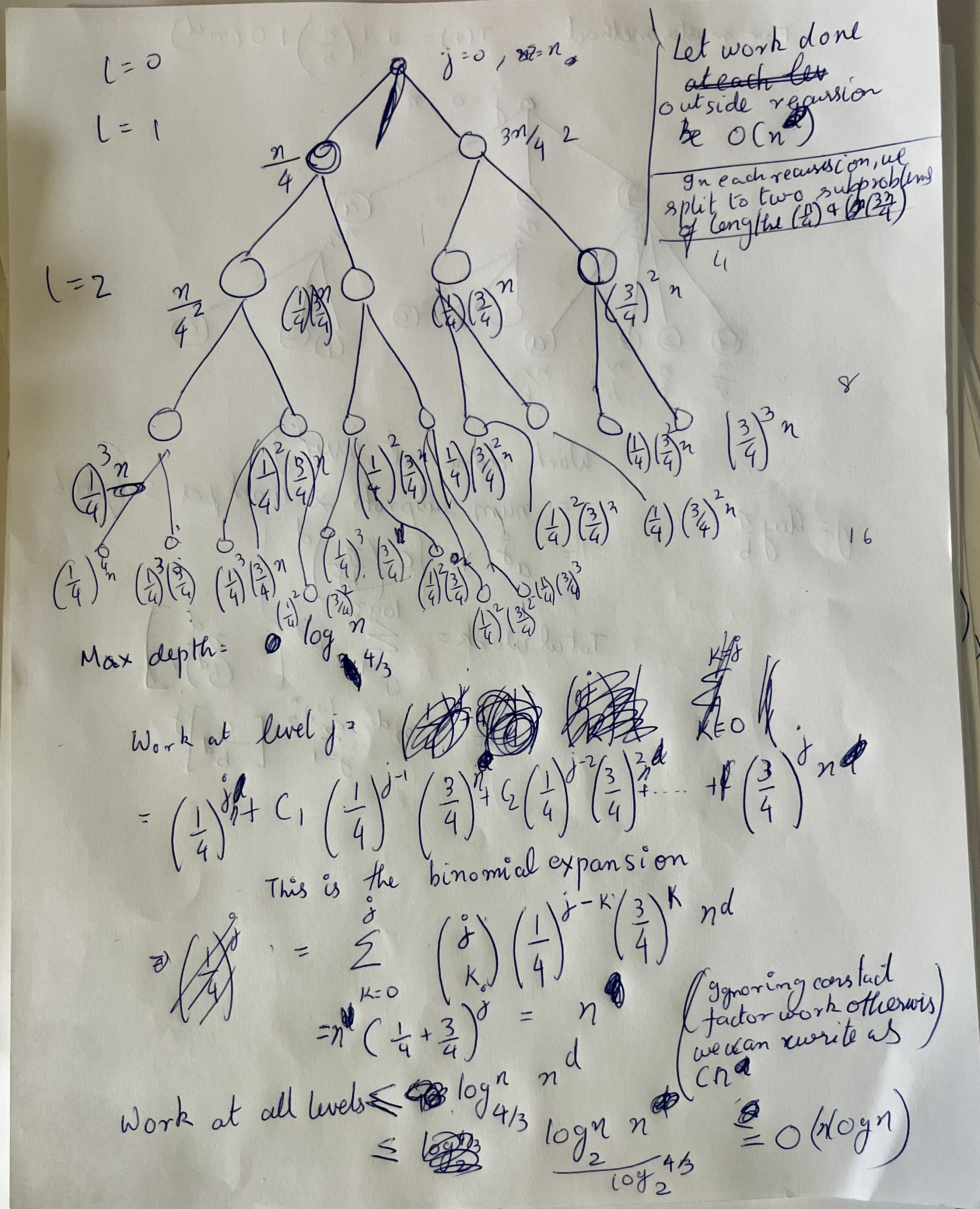
Even if we can choose a pivot that splits the problem into say 25-75 split, the run time will still be \(O(n \log n)\). We can prove this with recursion tree method and the binomial theorem.
import random

def quicksort(arr) -> None:
    """Sorts in-place"""
    qs_rec(arr=arr, lt=0, rt=len(arr)-1)

def qs_rec(arr, lt, rt):
    if lt >= rt:
        return
    # This partitions and places the pivot in the rightful place
    pivot_ix = partition(arr=arr, lt=lt, rt=rt)
    qs_rec(arr=arr, lt=lt, rt=pivot_ix-1)
    qs_rec(arr=arr, lt=pivot_ix+1, rt=rt)

def partition(arr, lt, rt):
    """Choosen a random pivot and partition the array such that all elements less than
    the pivot are to the left and greater than are to the right of the pivot.
    """
    # choose a random pivot and move it to the front
    pivot_ix = random.randint(lt, rt)
    pivot = arr[pivot_ix]
    arr[pivot_ix], arr[lt] = arr[lt], arr[pivot_ix]
    i = lt + 1  # first ix > pivot
    for j in range(lt + 1, rt + 1):
        if arr[j] <= pivot:  # arr[j] > pivot: do nothing
            arr[i], arr[j] = arr[j], arr[i]
            i += 1
    # swap the pivot to the correct position
    arr[lt], arr[i-1] = arr[i-1], arr[lt]
    return i-1

arr=[4, 5, 1, 1, 3, 1, 2, 0, 5, 7]
quicksort(arr)
print(arr)  # [0, 1, 1, 1, 2, 3, 4, 5, 5, 7]
Decomposition principle
To get time complexity of randomised algorithms
- Identify a random variable Y you care about
-
Express Y as a sum of indicator random variables \(Y = \sum_{e=0}^m X_e\)
- Apply linearity of expectation: \(E[Y] = \sum_{e=0}^m P[X_e = 1]\)
Selection problem
Given an array A with n distinct numbers and k, return the kth order statistic. The k-th order statistic is the kth smallest number.
10, 8, 2, 4 -> 3rd order statistic is 8. First order statistic is 2.
The solution is O(n). Using reduction, we can sort the array in O(n log n) by sorting and returning the (k-x1)th element.
Randomised
Follows quicksort almost verbatim.
Algorithm:
- Randomly choose a pivot and apply the partition subroutine from quicksort
- If the index of the pivot is k, return the value at the pivot.
- If the index of the pivot is greater than k (kth order statistic), then recurse on the left half of the array, otherwise recurse on the right half of the array.
Time complexity This is a linear time algorithm on expectation. The proof involves using
- Number of phases. A phase is where the input array is reduced to at least (3/4)th the input size. Phase j=0, we are processing an array of size btw, \(\left(\frac{3}{4}\right)^1 n\) and \(\left(\frac{3}{4}\right)^0 n\). Phase two (j=1), an array of size btw \(\left(\frac{3}{4}\right)^2 n\) and \(\left(\frac{3}{4}\right)^1 n\).
- Expected number of recursions to leave a phase (2). Because 50% of numbers result in a 25/75 split, it’s the same as the expected number of tosses of a coin before we see a head \(E[n] = 1 + 0.5E[n]\). This is because we need at least one toss. With 0.5 probability we are back to square one.
- Then total work becomes upper bounded by \(2 \times c \times n \sum_j \left( \frac{3}{4}\right)^j\). The infinite geometric sum is \(\frac{1}{1-r} = \frac{1}{1-\frac{3}{4}} = 4\). The total work becomes upper bounded by \(8cn\).
Deterministic - Median of medians
The algorithm is precisely the same as the randomised approach except how we choose our pivots. This algorithm is deterministically guaranteed to be of \(O(n)\). However, we pay in terms of very large constants in the big-O notation, need for an extra storage of length \(O\left(\frac{n}{5}\right)\).
Algorithm
- First split the array into n/5 buckets of sizes 5 each. For each bucket find the median through sorting.
- Store these medians in a new list.
- Then find the median of these medians by recursively calling this function.
- Once we have the pivot the rest is the same as the randomised selection.
Time complexity
- We need to notice that after each round, the pivot is guaraneed to shrink the array by at least 30% each time. Say we have 100 elements in the array. We split into 20 buckets and arrive at 20 medians. Then we find the median of these medians (M). This will point to say the 11th bucket. This means, there are 10 medians smaller than this (by definition). For each bucket these 10 medians belong to there are 3 elements (including the bucket median) smaller than the median of medians (M). That is there are 30 elements out of the 100 smaller than the median of medians (M).
- Next we write out the recurrence as \(T(n) = cn + T\left(\frac{n}{5}\right) + T\left(\frac{7n}{10}\right)\). We can then prove this with induction or a recursion tree approach.
Binary Search Tree (BST)
A balanced binary search tree can be thought of as a dynamic sorted list which supports insertions and deletions in \(O(\log(n))\) time when a sorted list would take \(O(n)\).
Binary Search Tree Property (balanced or otherwise): All the nodes in left subtree of a node n
are <= to n.val and all the nodes in the right subtree of n are
> the n.val. \(n_l.val <= n.val < n_r.val\). This is true for all the nodes
in the BST.
The height/depth of a BST can be anywhere between \(O(n)\) and \(O(\log_2(n))\) depending on if it’s balanced. So most operations are \(\theta(height)\).
Operations
        3
    /       \
    1       5
     \      /
     2     4
- To search for an element we start from the root and recurse/traverse to the left or the right depending on if the number is smaller or larger respectively than the current node. TC is \(\theta(height)\).
- Insertion is identical to search but we add the new node when the search terminates at a Null node. In case of duplicates, we take the conversion of adding to the rightmost position of the left subtree left of the matching node. TC is \(\theta(height)\).
- To find the minimum, we traverse to the leftmost element and similarly to find the maximum to traverse to the rightmost element of the tree. TC is \(\theta(height)\).
- To find the predecessor to a node
- If the node has a left subtree, then we find the maximum value in the left subtree.
- If it doesn’t, we move up parents until we find a parent that is smaller than
the query node. For instance, in the example above, for finding the predecessor
of
4, we go up to5but it’s larger than4, so we continue up to3which is smaller than4and this is indeed the4’s predecessor. Another way to think about this is we find the predecessor parent, when we turn left, ie., the current node is in the right subtree of an ancestor node. If you can never turn left, then you are the smallest element. Think of1above.
- To find the successor to a node
- If the node has a right subtree, then the smallest (leftmost) element contains the successor.
- If the node doesn’t have a right subtree, we walk up the parents until we find the first parent larger than the query node.
- Select i-th order statistic and Rank:
We will need to augment the tree withsize(n)in each noden. Thesize(n) = 1 + size(left) + size(right). The size of a null node is considered zero. The size is essentially the number nodes in the subtree rooted atn.
Select i-th order statistic:- We see if
size(left) = i-1, then the current node is the i-th order statistic. - If
size(left) >= i, we recurse left looking for thei-thorder statistic. - If
size(left) < i, then we recurse right looking fori - (size(left)+1).
Rank of node
n:
We recurse and find the noden. Every time you move left you add size(left)+1 to the running count until you reach the node you’re looking for. In the example below, say I want to find the rank of5, I start at the root2and move rt to 6. My running countr += size(1) + 1 = 2. Then I recurse left to4, nothing is added tor. Then I recurse to the right to5and addr += size(3) + 1 = 4. We returnr + 1.2 / \ 1 6 / 4 / \ 3 5 - We see if
Deletion has 3 cases:
- Leaf: No children. Simply mark the parent’s left/right pointer to
None. - One child: Point the parent’s left/right pointer (where the node to be deleted sits) to the single child of the node to be deleted.
-
Two children: This is quite cheeky. We run the predecessor operation which will will be the rightmost child of the left subtree (which is guaranteed to exist as this node has 2 children). Then we swap this node with the predecessor node (copy over children and parent pointers). This
  Delete 6 in the BST below
          3
      /       \
     1         6
             /    \
            5      7
          /
          4

  Step 1: Swap with predecessor (temporarily break BST invariant)
          3
      /       \
     1         5
             /    \
            6      7
           /
          4
  Step 2: Delete 6, we know how to deal with deleting nodes with single
  children. Simply move 4 up to be 5's left child.
          3
      /       \
     1         5
             /    \
            4      7
from dataclasses import dataclass

@dataclass
class Node:
    val: float
    lt: Optional['Node'] = None
    rt: Optional['Node'] = None

def inorder(node: Node) -> None:
    if node is None:
        return
    inorder(node.lt)
    print(node.val)
    inorder(node.rt)
Binary search
Insort
def insort(a, x):
    n = len(a)
    lt, rt = 0, n - 1
    while lt <= rt:
        mid = (lt + rt) // 2
        if a[mid] == x:
            rt = mid
            break
        elif a[mid] > x:
            rt = mid - 1
        else:
            # a[mid] < x:
            lt = mid + 1
    a.insert(rt+1, x)
    return a

 a = [1,2,3,4,5]

 insort(a, 2.3)
 insort(a, 88)
 insort(a, 0)
 insort(a, 4.5)
 # Out:  [0, 1, 2, 2.3, 3, 4, 4.5, 5, 88]