Table of Contents
- Foreword
- Activation and gradients
- Initialisations to prevent saturation of non-linear activations
- Batch norm
- Diagnostics
Foreword
These are notes taken from Andrej Karpathy’s lecture “Building makemore Part 3: Activations & Gradients, BatchNorm”. Full lecture series: youtube.
Here’s the Jupyter notebook with code for the plots below.
Activation and gradients
The following assumes you are building a classification model with a simple Multi-Layer Perceptron (MLP). That is you have repeated linear followed by some nonlinear activation (ex. \(\tanh\)) layers predicting logits of the output classes. The final logit layer goes through a softmax and cross entropy loss function.
For the sake of simplicty assume a model like below
\[\begin{align*} x_0 &- \text{input}\\ x_1 &= tanh(x_0 W_1 + b_1)\\ x_2 &= x_1 W_2 + b_2\\ y &= softmax(x_2)\\ loss &= \text{cross_entropy}(y, y^{true}) \end{align*}\]Forcing last layer of softmax to not be so confidently wrong
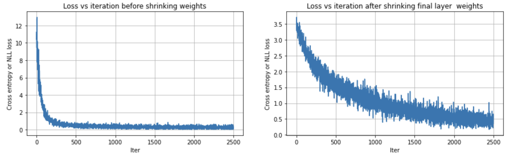
We do this by making the weight matrix of the final logits layer to be close to zero. The logits consequently become closer to zero, ie., roughly equal. After softmax, the probabilities are roughly equal, ie., \(\frac{1}{\text{output_size}}\). Remember the loss is only derived from the true class label. It’s better to get a smaller loss by going with \(\frac{1}{\text{output_size}}\), instead of strongly choosing another class. This prevents the elbow/hockeystick loss graph and wasting a couple of training rounds.
The below shows applying this improvement for the makemore problem explained in this youtube video.
Initialisations to prevent saturation of non-linear activations
If the initialisation moves the activations to the saturated regions, the gradients don’t flow back (vanishes). The gradient at saturation points are roughly 0 because small perturbations in the saturation region will have no impact to the output and loss function. Or equally the slope at the saturations is roughly 0. This also leads to dead neurons.
Dead neuron
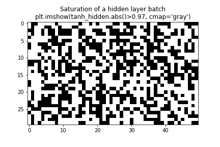
A dead neuron is one where the neuron initialised in a region where it’s always saturated for all training inputs. In this scenario the neuron never receives a non-zero gradient and never learns. One way to quickly notice dead neurons is to imshow activations of a batch and see if a specific neuron is saturated in the entire batch.
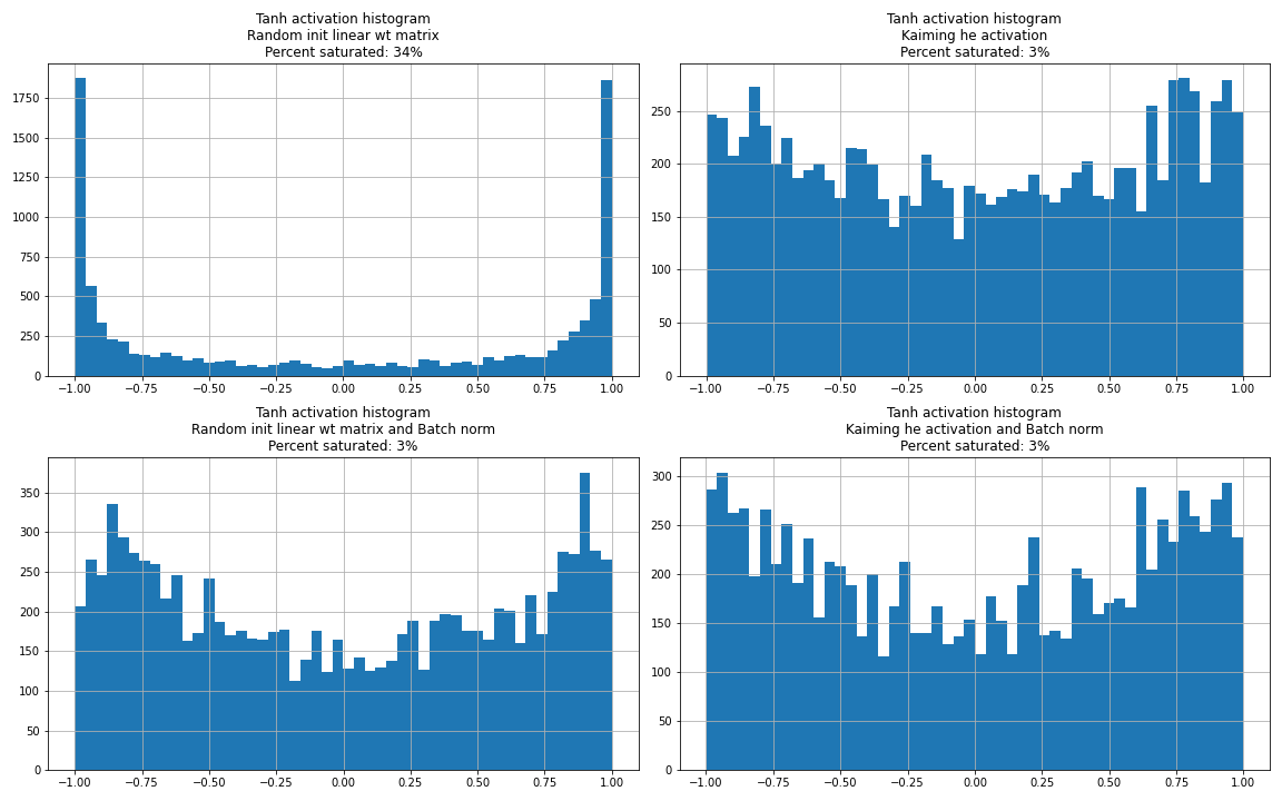
Kaiming He activation
One solution is to initialise the weights in the correct scale. If the input to the \(\tanh\) is in the region around 0 and not too spread out we will not have saturations. Pytorch uses the Kaiming He initialisation. They sample from a uniform distribution between \(\left(-\frac{\text{gain}} {\sqrt{\text{fan_in}}},\frac{\text{gain}} {\sqrt{\text{fan_in}}}\right)\). This makes the input to the nonlinearity to lie in the non-saturated regions. This also makes the gradients roughly gaussian (no extreme gradients ie., not a wide gaussian).
\(tanh\) is a squashing function and it can only shrink the gradients. This squashing property is also the reason we have a gain when we sample. For \(tanh\) the empirical gain is (5/3) and for ReLU it’s \(\sqrt{2}\) as half of the space is squashed to 0. If we simply stacked linear layers, we wouldn’t need the gain. Without the gain the output of deeper layers start squishing down to 0. The deeper you go the higher the issue.
From pouannes blog: The only difference is that the Kaiming paper takes into account the activation function, whereas Xavier does not (or rather, Xavier approximates the derivative at 0 of the activation function by 1).
Batch norm
The above careful initialisation is not practical for very deep neural nets. Instead we force the input to the non-linearity to be a unit gaussian. We mean center and divide by the standard deviation of the output of the linear layer from the batch. However, we want the to allow the model to saturate some neurons and shift the mean. Hence, we later multiply with \(\gamma\) (scale) of dimensions fanout with the output of the standardised linear layer and add \(\beta\) (shift). These are trained by the model. This guarantees the input to the \(tanh\) or nonlinearity is roughly gaussian at least at the beginning of the training.
This makes the model more robust to initialisation in terms of output of nonlinearity and gradients. However, different initialisation scale will still need different learning-rate.
The fact that the forward pass depends on other samples in the batch has a regularising effect (entropy is good in training). When using batch norm, we remove the bias term from the linear or convolution layer. This is because the bias is a redundant as it will eventually be removed when we subtract the mean in the Batch Norm.
In order to not derive the mean and std in inference we compute a running variance and mean during training with an exponential smoothing (the smoothing ratio is called momentum in pytorch).
Batch norm is finicky and can lead to a number of bugs. It’s hard to get rid off as it works well both from the optimisation and the regularisation perspective. People have developed other normalisation techniques such as layer, group, and instance normalisation.
We don’t get a complete free pass. If the scales of the weight matrices change, even with batch norm, we will have to tune the learning rates.
Diagnostics
Saturated neurons image
This is as described in the dead neurons section.
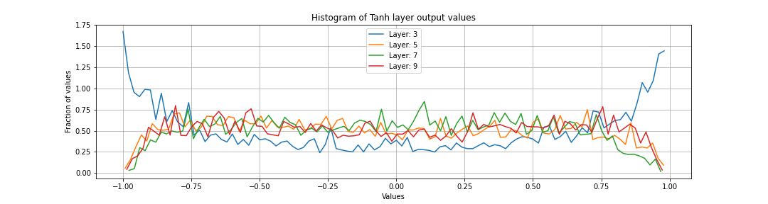
Activation histogram
We want only a small proportions of the neurons to be saturated.
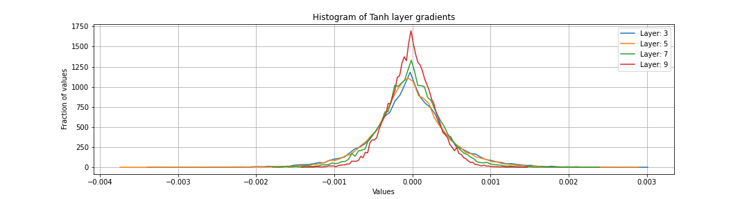
Gradient of activations histogram
We want the gradient of all layers to be roughly the same gaussian. We don’t want the gradients to be shrinking or exploding. If weight gain used while initialising Weight matrices of linear (without batch norm) is too small or too large, we will see the shrinking or the exploding phenomenon. Before batch normalisation, it was incredibly tricky to set the right initalisations so that the gradients don’t explode or vanish.
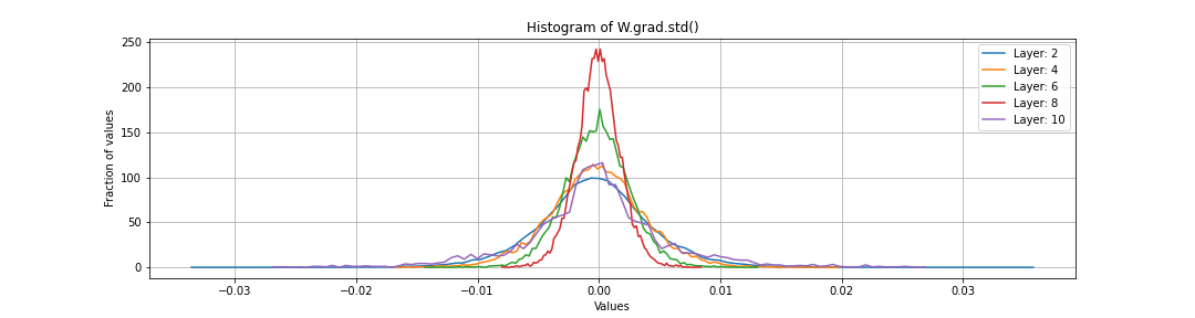
Gradient of the weight matrices W.grad
In addition to a histogram of W.grad, also instructive to look at W.grad.std()/W.data.std(). This is because we are using these gradients to update the weight matrix values and we want them to be at the right scale. Specifically, if the gradients are too large wrt to the scale of the weights, we are in trouble. Because we artificially shrunk the weights of the last logits layer close to zero, we would expect very large gradients wrt to it’s scale. However, this usually will fix itself after a few rounds of training.
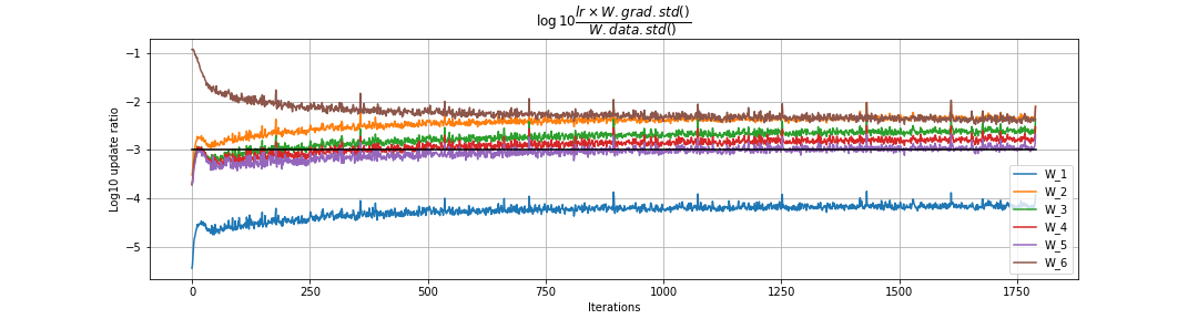
Ratio of updates to weight matrices to the weight matrix data
We are measuring
\[\dfrac{\text{update.std()}}{\text{param_value.std()}}\] \[\log10 \dfrac{ lr \times W.grad.std()}{W.data.std()}\]We plot this ratio in the \(\log10\) scale on the y axis and the training round on the x-axis. We cannot see the trend in a single run; we need to run the training for a few rounds (say 1000). Rule of thumb is that update should be roughly \(10^{-3}\) or \(-3\) in the \(\log10\) scale.