Minimising Cross Entropy =
Minimising KL-Divergence?

Table of Contents

1. Entropy & KL-Divergence
   1. Entropy summary
   2. Cross entropy
   3. KL-Divergence
   4. Why is minimising Cross-Entropy or KL-Div, the same?
2. Which one should you use in production? Normalised Cross Entropy
   1. Real world example of cross entropy interpretation issues
   2. Normalised Cross Entropy
   3. Why not KL-Divergence?
3. Appendix: Entropy through graphs and pictures

Entropy & KL-Divergence

Entropy summary

Measures the uncertainty in a system. It can also be thought of as the amount of surprise. In an information theoretic view, it’s the amount of information needed to remove the uncertainty in the system.

Above we are sampling \(x\) from the distribution \(P(x)\): that is the probability of sampling the specific value \(x\) is defined by the probability distribution \(P(x)\).

This medium blog post works through examples that might be instructive.

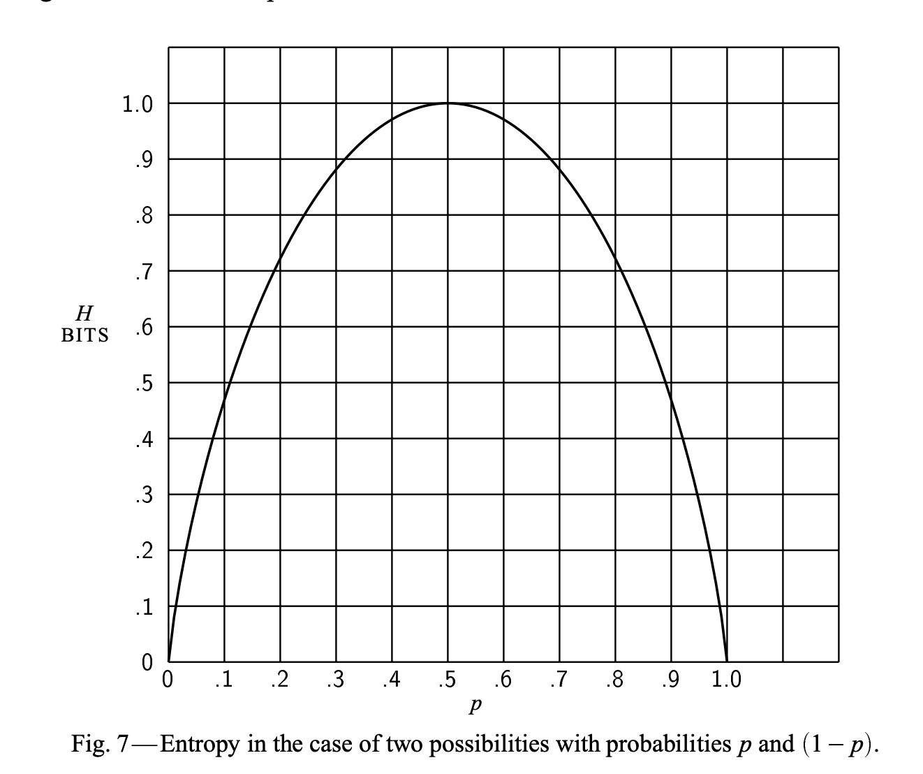
Entropy is a non-negative real number. Entropy is bounded between 0 and 1 when there are only two outcomes. However, if there are more outcomes it can be greater than 1. In ML parlance, for a binary output variable Y, entropy can be at most 1 but for a multiclass setup, it can be greater than 1.

Cross entropy

This is the entropy of a distribution \(q(x)\) when \(x\) is sampled from another distribution \(p(x)\).

In ML, \(p(x)\) represents the true unknown distribution we are trying to model with \(q(x)\). We never really have access to the true distribution \(p(x)\), but only \(X\), our dataset sampled from \(p(x)\). Here \(X\) represents the entire dataset, \(X\) and \(y\) in supervised learning, not just the features. When we actually go about computing cross entropy, we merely compute the average \(\log q(x)\) with \(x\)’s sampled from our data. This is an unbiased estimate of the true cross entropy of \(q(x)\) wrt \(p(x)\).

import numpy as np
import numpy.typing as npt

Vector = npt.NDArray[np.float64]

# Penalty for the model q(x) for estimating 0 probability of seeing a sample x
# from p(x).
LARGE_PENALTY = -100

def q(x: Vector) -> Vector:
    model = fetch_model()
    return model.probability_of_x(x)

def cross_entropy(qx: Vector) -> float:
    logs = np.log(qx)
    logs[logs==-np.inf] = LARGE_PENALTY
    return -logs.mean()

X: Vector = sample_from_true_distrbn_p_of_x(size=100)
print(cross_entropy(qx=q(x=X)))

KL-Divergence

Read the treatise on KL-D from UIUC.

KL Divergence is a measure of closeness of two distributions. It is not a distance metric as it is asymmetric, more concretely, \(D_{KL}(p(x)||q(x)) \neq D_{KL}(q(x)||p(x))\). As mentioned above, in ML \(q(x)\) is usually the model we are building to approximate the true distribution \(p(x)\).

Discrete case

Continuous case

If \(p(x) \neq 0\) for some \(x \in X\), but \(q(x) = 0\), then \(D_{KL} = p(x) (\log p(x) - \log 0) = \infty\). If there’s a point which has non-zero probability in the true distribution that the model distribution thinks is impossible, then the two distributions are considered absolutely different. This can be addressed by smoothing. See the UIUC notes for more details.

Why is minimising Cross-Entropy or KL-Div, the same?

Credits: stats.stackexchange

Cross-entropy is the loss function used in logistic regression.

Hence, we can decompose KL-Divergence into the entropy of the true unknown distribution \(p(x)\) plus the cross entropy of \(q(x)\) with respect to the true distribution \(p(x)\). While learning a model, we try to figure out the parameters \(\left(\Theta\right)\) of our model defining \(q_{\Theta}(x)\) which minimises our loss. The parameters of the model do not affect the true probability distribution \(p(x)\), so

import torch
import torch.nn.functional as F
import numpy as np

def create_y(num_data: int, num_classes: int) -> np.ndarray:
    """Creates a random class probability labels.

    :returns: A ``num_data x num_classes`` matrix such
        that each row sums to 1 (corresponds to probabilities).
    """
    y = np.random.random((num_data, num_classes))
    return y / y.sum(axis=1)[:,None]

def cross_entropy(y_true: np.ndarray, y_pred: np.ndarray) -> float:
    """"Computes multiclass cross entropy.

    :param y_true: A matrix of dimenions (n, m), for n datapoints and
        m labels. True class labels. Can be OHE or probabilities.
    :param y_pred: A matrix of dimensions (n, m) with prediction probabilities for
        the n-datapoints for the m-classes. We will assume that all probabilities are > 0.
    """
    return (- y_true * np.log(y_pred)).sum(axis=1).mean()

def kl_divergence(y_true: np.ndarray, y_pred: np.ndarray) -> float:
    """Computes the KL-Divergence btw true and predicted class labels"""
    return (
        - cross_entropy(y_true, y_true)
        + cross_entropy(y_true, y_pred)
    )

# Test our implementation
y_true = create_y(100, 4)
y_pred = create_y(100, 4)
print(cross_entropy(y_true=y_true, y_pred=y_pred))
# Output: 1.59156
print(kl_divergence(y_true=y_true, y_pred=y_pred))
# Output: 0.3567

# Verify with implementation in pytorch
y_true_tnsr = torch.from_numpy(y_true)
y_pred_tnsr = torch.from_numpy(y_pred)
print(F.cross_entropy(input=torch.log(y_pred_tnsr), target=y_true_tnsr))
# Output: tensor(1.5916, dtype=torch.float64)

Which one should you use in production? Normalised Cross Entropy

Well honestly, you can track either KL-Divergence \(D_{KL}\) or Cross entropy \(H\) in production. Minimising either loss is identical as we have seen above.

However, KL-Divergence is slightly easier to reason with.

Let’s say we have a perfect model such that \(q(x) = p(x) \forall x \in X\). Cross entropy \(H(p, q)\) will be non zero whereas KL-Divergence will be zero \(D_{KL}(p, q)\). For a concrete example, say for \(p(x=0)=p(x=1)=0.5\) and hence \(q(x=0)=q(x=1)=0.5\), cross entropy will be \(H(p, q) = - p(x) \log q(x) = - 2 \times (0.5 \log 0.5) = 0.7\), whereas KL-Divergence will be \(D_{KL}(p, q) = E[\log p] + H(p, q) = -0.7 + 0.7 = 0\).

Real world example of cross entropy interpretation issues

Say we are modelling the probability that the user clicks on an ad (or the Ads Click through Rate). We want to build two models one on the home page and one on a search page. Let’s say that users are more likely to click on ads on the search page than the home page, such that the \(P(click=True \mid page=home) = 0.1\) and \(P(click=True \mid page=search) = 0.3\).

Now we come up with the simplest model possible, a model that predicts the average click through rate every time which is (\(0.1\) for home and \(0.3\) for search). We collected 100 visits to our home page and 100 visits to our search page which resulted in 10 and 30 ad clicks respectively. We want to compute the model performance in terms of cross entropy.

Does that mean our homepage model is twice as good as the searchpage model? Well intuitively we want to say no. We see that cross entropy value is highest when the probability of the binary number variable is 0.5 and we predict 0.5 for all the samples. This makes comparing models difficult with cross entropy. Note: KL-Divergence of the above example will be 0.

Normalised Cross Entropy

As discussed above cross entorpy is hard to reason about. Is a cross entropy of 0.3 good? Who knows?! The standard trick to arrive at numbers that we can intuit about is to normalise.

From the literature, we see that Normalised Cross Entropy is used widely in the industry. Normalised Cross Entropy is the ratio of your model’s cross entropy over the cross entropy of a model that simply predicts the mean of the labels.

The smaller the number the better. The idea is that the denominator is predicting the average and if your model is doing worse using features than predicting the average class probability then you are overfitting to noise and you are better off just predicting the average. For the homepage and searchpage example discussed above this will be 1 in both cases.

where \(p_i\) is the estimated \(P(y_i=1 \mid X=x_i)\) and \(p=\frac{\sum_i y_i}{N}\) is the mean of \(Y\).

def normalised_cross_entropy(y_true: np.ndarray, y_pred: np.ndarray) -> float:
    model_cross_entropy = cross_entropy(y_true=y_true, y_pred=y_pred)
    y_pred_baseline = y_true.mean() * np.ones_like(y_pred)
    baseline_cross_entropy = cross_entropy(y_true=y_true, y_pred=y_pred_baseline)
    return model_cross_entropy / baseline_cross_entropy

Why not KL-Divergence?

Well honestly it’s still difficult to intuit about values of KL-Divergence. Is a KL-Divergence of 0.3 good? I don’t know. I find Normalised Cross Entropy easy to reason about when comparing model performance. Nothing is stopping us from normalising KL-Divergence by dividing with the KL-Divergence of the mean prediction similar to Cross Entropy but I haven’t seen it in the literature as much. In my opinion, this could work just as well.

Appendix: Entropy through graphs and pictures

Below is a plot of \(- \log x\). So an event \(x\) which has a probability of 1, will have a surprise of 0 or equally in an optimal coding, we will use 0 bits to communicate this event. If an event has a probability close to 0, seeing this event will produce a very large amount of surprise or it makes sense in an optimal coding to use a large number of bits to represent this rare event.

This definition of entropy was proposed by Claude Shannon in the paper A Mathematical Theory of Communication. He shows that only a function of the form \(-K \sum_i p_i \log p_i\) satisfies the the three requirements he places for entropy. See section 6 of the paper for details.

Here’s a jupyter notebook with visualisation of entropy as a function of how spread out a distribution is.