Multivariate Calculus

Table of Contents

1. Acknowledgement
2. Gradient
3. Total derivative
4. Jacobian
5. Hessian
6. Real world is painful
7. Multivariate chain rule
8. Backprop
9. Activation functions in NN
10. Optimisation: Linearlisation, Power Series and Taylor Series
11. Gradient descent
12. Lagrange multipliers & constrained optimisation
13. Learnings from implementing gradient
14. Gradient CheatSheet
15. Advanced optimisation techniques
16. Convex optimisation

Acknowledgement

Notes are partially derived from ICL’s course on coursera.

Cheatsheet from ICL. Skip to Gradient Cheatsheet for if you just want the vector calculus formulas.

Gradient

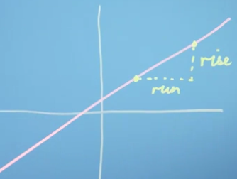
To compute the tangent or slope at a point, draw a straight line perpendicular to the curve. Take any points on this slope line and divide the value of the function at this point by distance between the points.

Example

Total derivative

Imagine you want to find the rate of change of temperature faced by a particle wrt to time. The temperature in the space does not change with time, however the particle is moving in space. So, temperature is a function of x, y, z and these are functions of t.

Jacobian

If you have \(f(x_1, x_2, x_3, ..., x_n)\), the Jacobian \(J\) is given by \(J = \begin{bmatrix} \dfrac{\partial f}{\partial x_1}, \dfrac{\partial f}{\partial x_2}, \dfrac{\partial f}{\partial x_3}, ..., \dfrac{\partial f}{\partial x_n}\end{bmatrix}\). As a convention this is written as a row vector.

Example: \(f = xy^2 + 2z\)

The Jacobian can be thought of as an algebraic expression for a vector, which when give a specific \(x, y, z\) coordinate will return a vector pointing in the direction of the steepest slope for this function at \(x, y, z\). This function has a constant contribution in the \(z\) direction independent of the \(x,y,z\) location chosen.

Jacobian is a vector pointing in the direction of the steepest uphill slope. The steeper the slope, greater the magnitude of the Jacobian at the point.

Jacobian and linear transformation

Say we are going from cartesian space \((x, y)\) to polar coordinates \((r, \theta)\), then \(x=r cos\theta\) and \(y = r sin \theta\).

Though the transformation is clearly non-linear, as a consequence of the transformation being smooth, the areas only depend on \(r\) and not \(\theta\), consequently can be closely approximated as linear.

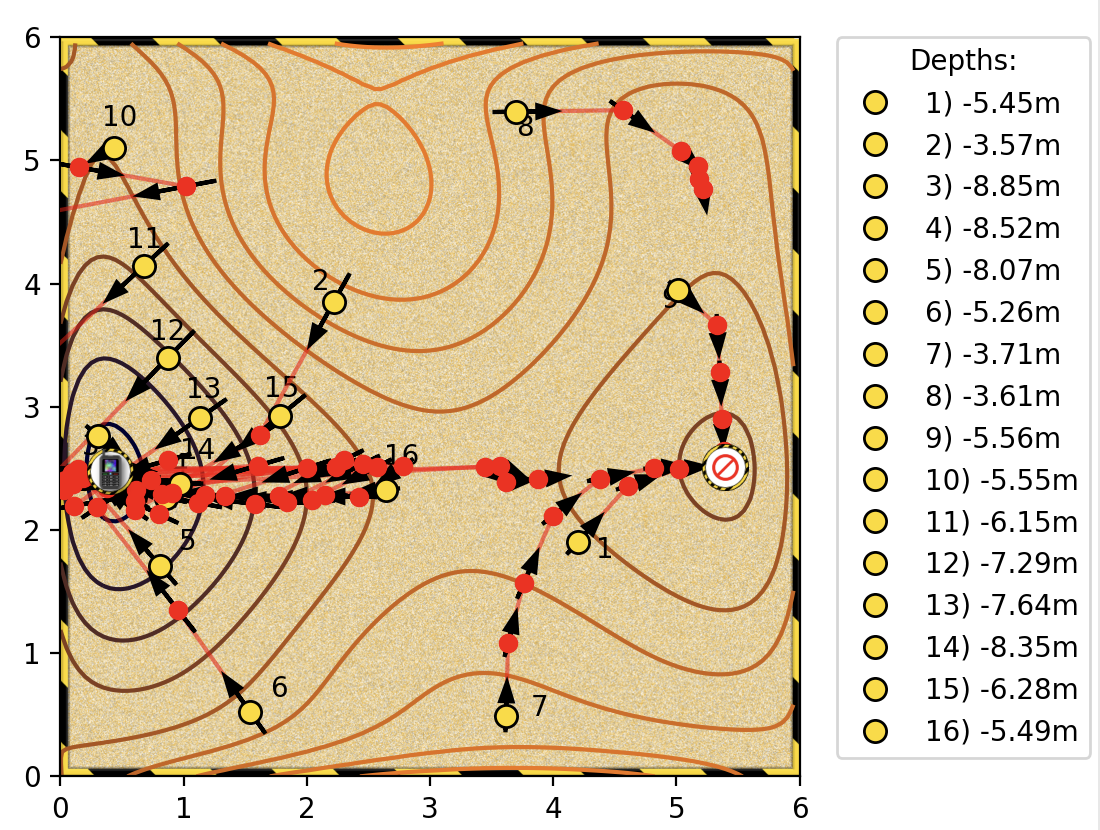
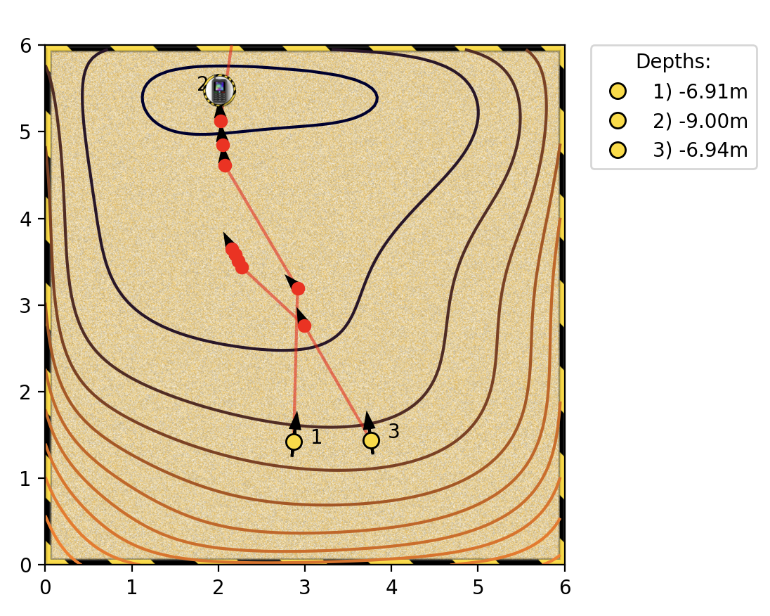
Optima search with Jacobian

Notes based on the sandpit excercise. We manually try to find the optimal by clicking on various points in a sandpit.

The following scenarios are easier to solve.

• Analytically simple expressions for the objective function. We set the jacobian to zero and find the optimal points.
• Lower dimensions (say 2 dimensions). We can literally sample the space as a 2D grid and find the maximas and minimas.
• Convex: many convex optimisation tools

Nonconvex objective function. Helps to (randomly) sample a wide region of the space before we hill climb lest we get trapped in a local optima. Gradient is far more efficient once we’ve narrowed down a space to hill climb. Sampling and evaluating the function is time consuming.

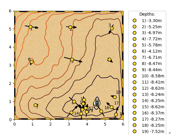
Irregular (non-smooth) surfaces in the objective function lead to noisy gradients, making it difficult to trust the direction of steepest slope based on a single gradient.

Hessian

Second order derivative of a function of n variables. Apply the Jacobian to the Jacobian. For the function \(f(x, y, z)\)

The Hessian is symmetric. There is a relationship between the Hessian and the covariance/fisher information matrix (outside the scope of this doc).

Hessian examples

\(f = x^2 + y^2 , J = \begin{bmatrix} 2x & 2y \end{bmatrix} , H = \begin{bmatrix} 2 & 0 \\ 0 & 2 \end{bmatrix}, |H| =4\)

This function clearly has circular contours with f=(0,0) being the minima. It’s easy to see that at \(x=0, y=0, J =0\), hence this has to be an optima.

If the determinant of the hessian is positive, then the point is either a minimum or a maximum. And if the first entry of the hessian is positive, it is a minimum. If the determinant is non-positive, we have a saddle point (inflection point). Example: \(x^2 - y^2\) at \((0, 0)\), \(\| H \| = -4\). See math.stackexchange for details.

Real world is painful

In real life, we often don’t have an analytical form for the objective function. We instead use the finite difference method (numerical methods) to approximate the gradient/hessian at a given starting point and continue hill climbing.

Also often the space can discontinuities (RELu function). Additionally, could have rough edges leading to untrustworthy gradients.

If \(\Delta\) is too large it will be a bad approximation, if too small we will have numerical issues (\(\Delta f\) will be a small divided by a small number \(\Delta x\)). One solution is to take the gradient at a few step sizes and take the average (sample around the point).

Multivariate chain rule

Let \(f(x_1, x_2, ..., x_n) = f(\mathbf{x})\)

Chaining vectors in differentiation

Let \(f(\mathbf{x}(\mathbf{u}(t)))\) \(\begin{align*} f(\mathbf{x}) &= f(x_1, x_2) \\ x(\mathbf{u})&=\begin{bmatrix} x_1(u_1, u_2) \\ x_2(u_1, u_2) \end{bmatrix}\\ u(t) &= \begin{bmatrix} u_1(t) \\ u_2(t) \end{bmatrix}\\ \frac{df}{dt} &= \frac{\partial f}{\partial \mathbf{x}}\frac{\partial \mathbf{x}}{\partial \mathbf{u}} \frac{d\mathbf{u}}{dt}\\ &= \begin{bmatrix} \frac{\partial f}{\partial x_1} & \frac{\partial f}{\partial x_2} \end{bmatrix} \begin{bmatrix} \frac{\partial x_1}{\partial u_1} & \frac{\partial x_1}{\partial u_2} \\ \frac{\partial x_2}{\partial u_1} & \frac{\partial x_2}{\partial u_2} \end{bmatrix} \begin{bmatrix} \frac{d u_1}{dt} \\ \frac{d u_2}{dt} \end{bmatrix} \\ &= J_{f\mathbf{x}} J_{\mathbf{xu}}J_{\mathbf{u}t} \end{align*}\)

Backprop

Simple 1-D example

We can simplify this by

For multivariate case

For n layers,

Activation functions in NN

Sigmoid

\(tanh\), logistic function, \(\sigma(\mathbf{z}) = \frac{1}{1 + \exp(-\mathbf{z})}\). For the logistic activation function, each output node is between 0-1 or can be thought of as a probability (bernoulli variable). However the sum of the probabilities of the last layer will clearly not be 1, each output refers to an individual probabilty or bernoulli variable. If you want a multi-class classifier or multinomial variable, then you can use the softmax function, \(\tau^{(L)} = exp(z^{(L)}), \widehat{y} = \dfrac{\tau^{(L)}}{\sum_{j}\tau^{(L)}_j}\) .

Grad of activation functions and the Hadamard product

If we choose, tanh or logistic activation function then \(\frac{\partial \mathbf{a}}{\partial \mathbf{z}}_{(n\times n)}=\sigma'(\mathbf{z})_{(n \times n)}\) is a diagonal matrix. This is because the activation of the i-th node of the output layer only depends on the \(z_i\). We can get away without constructing the diagonal matrix.

The \(\odot\) is the Hadamard product or the pointwise multiplication product.

This only applies to activation functions which are not dependent on the other nodes of the input.

Optimisation: Linearlisation, Power Series and Taylor Series

Summary

The idea here is to approximate the unknown objective function with a n-degree polynomial, usually 1st or 2nd degree polynomial. We minimise this polynomial iteratively moving closer to the minimum of the objective function. The hope is locally a smooth function behaves similar to a simpler polynomial function.

We find the \(\arg\min\) of the polynomial by differentiating it and solving the parameters for the derivative equal to zero. For a degree-1 polynomial the minimum is where the slope (\(f'(x_0)\)) is zero. We instead move in the direction steepest downward slope with some arbitrary step-size. For a degree-2 polynomial the minimum is exactly at \(\Delta x = -\frac{f'(x_0)}{f''(x_0)}\).

Power series approximations

\(g(x)\) is a power series, \(g(x) = a+bx+cx^2+\ldots\) Hope is to represent or approximate a general function \(f(x)\) with a polynomial function \(g(x)\).

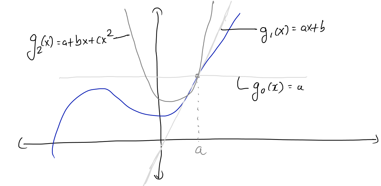
where \(g_0(x), g_1(x), g_2(x)\) are called the truncated series. These are the the zeroth, first and second order approximations respectively.

If you have a well-behaved function (smooth, ie., continuous and infinitely differentiable), then the value of the function anywhere can be derived by simply knowing the values of all the infinite differentials at any single point.

Taylor series

We can derive the taylor series to follow by essentially taking a polynomial, say \(g(x)= ax + b\), differentiating it once and setting it’s slope to the first derivate of the function \(f(x)\) at a point \(x_0\), \(a=f'(x_0)\). Now let’s take \(g(x) = ax^2 + bx + c\), differentiating twice and equating the second-derivative we get \(2a = f''(x_0)\). Doing this once more we get \((2)(3) a = f'''(x_0)\). It’s clear that the coefficient of the \(n-th\) power of the \(g(x)\) function is simply \(\frac{f^{(n)}(x_0)}{n!}\).

1-D

When \(a=0\), the Taylor series becomes the Maclaurin series.

More often this is expressed as

Rearranging,

we can see that if we use the finite difference method to approximate the gradient of a function (using the secant instead of the tangent), the error of our estimate of our gradient will be of the order \(O(\Delta x)\). This is because for the region near \(x\), \(\Delta x\) is small, hence highers powers of \(\Delta x\) and consequently higher order differentials will have increasingly diminishing contribution to the value of the function near \(x\).

2-D

For a 2-D, case we can explicitly write this out

It’s easy to see how the higher order terms will take on the binomial expansion form.

Multivariate

In a multivariate setting the taylor series can be extrapolated as

Newton-Raphson method

The below is just to inspire iterative methods.

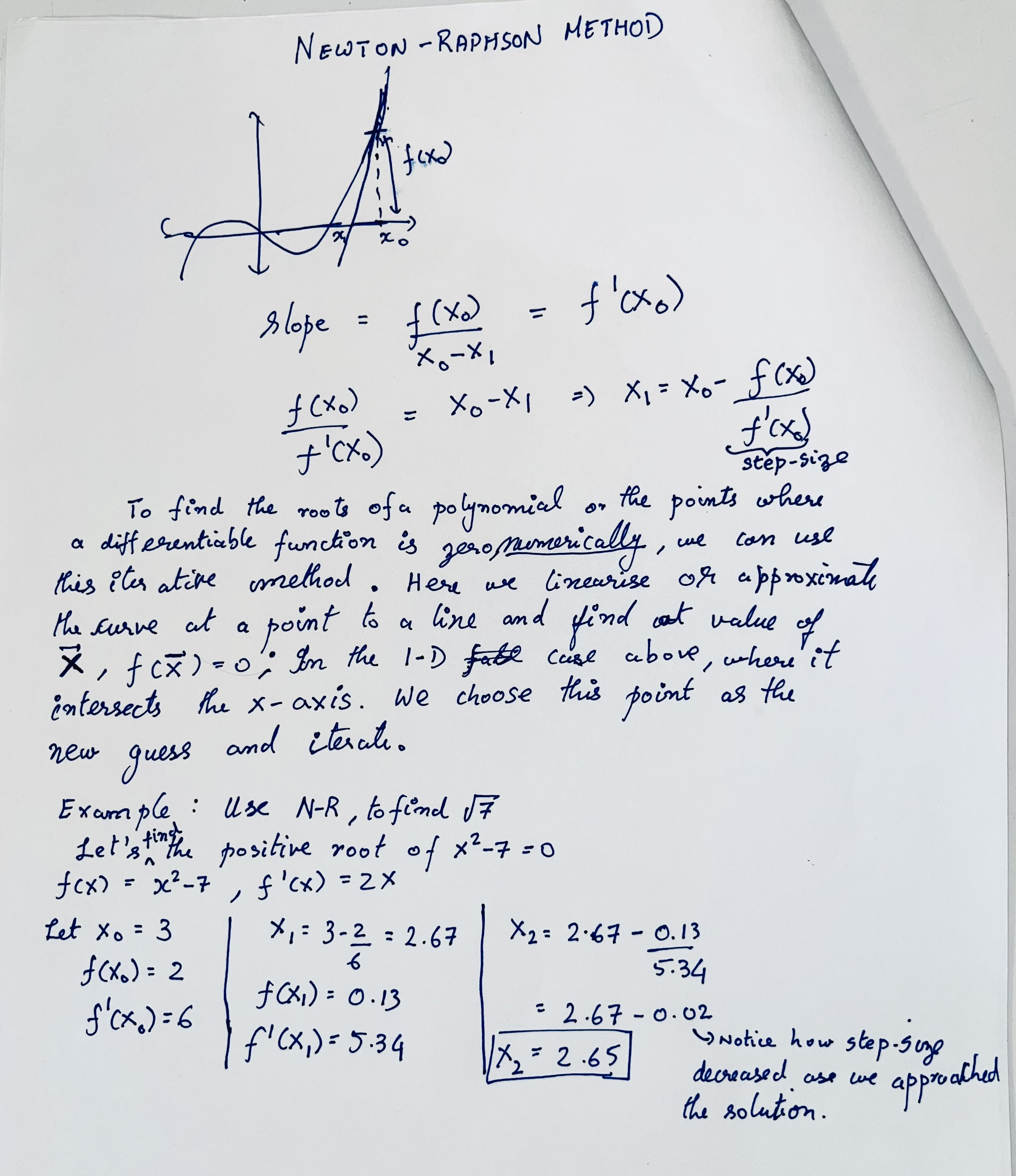
This method also applies to complex roots of a function.

Failure mode

If you begin your guess of the solution around a local minimum, then the iteration will get stuck and jiggle about the minimum until it escapes by chance. Some times this can form cycles where it will never get out.

With scipy

from scipy import optimize

def f(x):
    return x**2 + 2*x/3 - 7

optimize.newton(f, x0=2)

Gradient descent

Let \(f(\mathbf{x})\) be the objective function we are optimising (we want to find a minimum of this function).

First order

We want to move in the direction of the sleepest slope downwards. This is essentially the Gradient or the Jacobian of the function at this point.

We are approximating the function with a degree one polynomial. To find the mimumum of this function, let’s differentiate and set it to 0.

This is redundant. We have defined the minimum is where the slope (or grad) is 0.

\(\begin{align*} \mathbf{x}_{new} &= \mathbf{x}_{old} - \gamma J^T_{f@{\mathbf{x}_{old}}}\\ \mathbf{x}_{new} &= \mathbf{x}_{old} - \gamma \nabla_{f@{\mathbf{x}_{old}}} \end{align*}\)

Above we use the first-order approximation and follow the gradient down the slope. However since we don’t know how to set the step-size \(\gamma\) we can bounce around the optimum.

Second order

Using the Hessian we can automatically set the step size. This would lead us to either the maximum or the minimum.

We are approximating the function with a degree two polynomial (2nd order Taylor series expansion). To find the mimumum of this function, let’s differentiate and set it to 0. To make the math cleaner, let’s make the Jacobian a column vector.

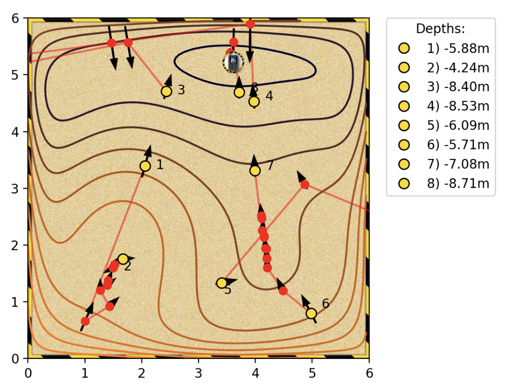
Hybrid method

If we are sufficiently close to a stationary point already, the Hessian method will find it in relatively few steps. Though in most cases, the step size is too large, and can even change the direction up hill.

We can try a hybrid method which tries the Hessian unless the step would be too big, or it would point backwards, in which case it goes back to using steepest descent.

def next_step(f, J, H) :
    gamma = 0.5
    step = -linalg.inv(H) @ J
    if step @ -J <= 0 or linalg.norm(step) > 2 :
        step = -gamma * J
    return step

Lagrange multipliers & constrained optimisation

This video from Texas A&M is quite instructive.

Say we have an objective function \(f(x,y)=x^2y\) that we would like to optimise. However, we would like to constraint to solutions which lie on the circle \(g(x,y)=x^2+y^2=a^2\). Lagrange noticed that this happens when the surface of the objective function \(f(x,y)\) and the constraint function \(g(x,y)\) just touch each other. That is the gradient of the functions are pointing the in same or the opposite direction. Imagine a small sphere touching either the inside or the outside of a larger sphere.

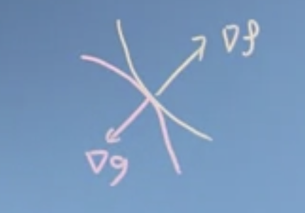
The above observation can be formalised as \(\nabla f = \lambda \nabla g\), where \(\lambda\) is called the lagrange multiplier. In the above example

So through the grads, we had two equations with 3 unknowns, \(x, y\) and \(\lambda\). But we had one equation from the constraint \(g(x)\).

Another way to write the above would be to find the roots of the following equation.

In other words, in a 3-D parameter space of \((x, y, \lambda)\) , we want to find where \(\nabla L(x, y, \lambda)\) goes to zero. We can find this with root finding algorithms like Newton-Raphson.

\(\nabla \mathcal{L}\) because it can be written as the gradient (over \(x, y,\) and \(\lambda\)) of a scalar function \(\mathcal{L}(\mathbf{x} \lambda)= f(\mathbf{x})− \lambda g(\mathbf{x})\).

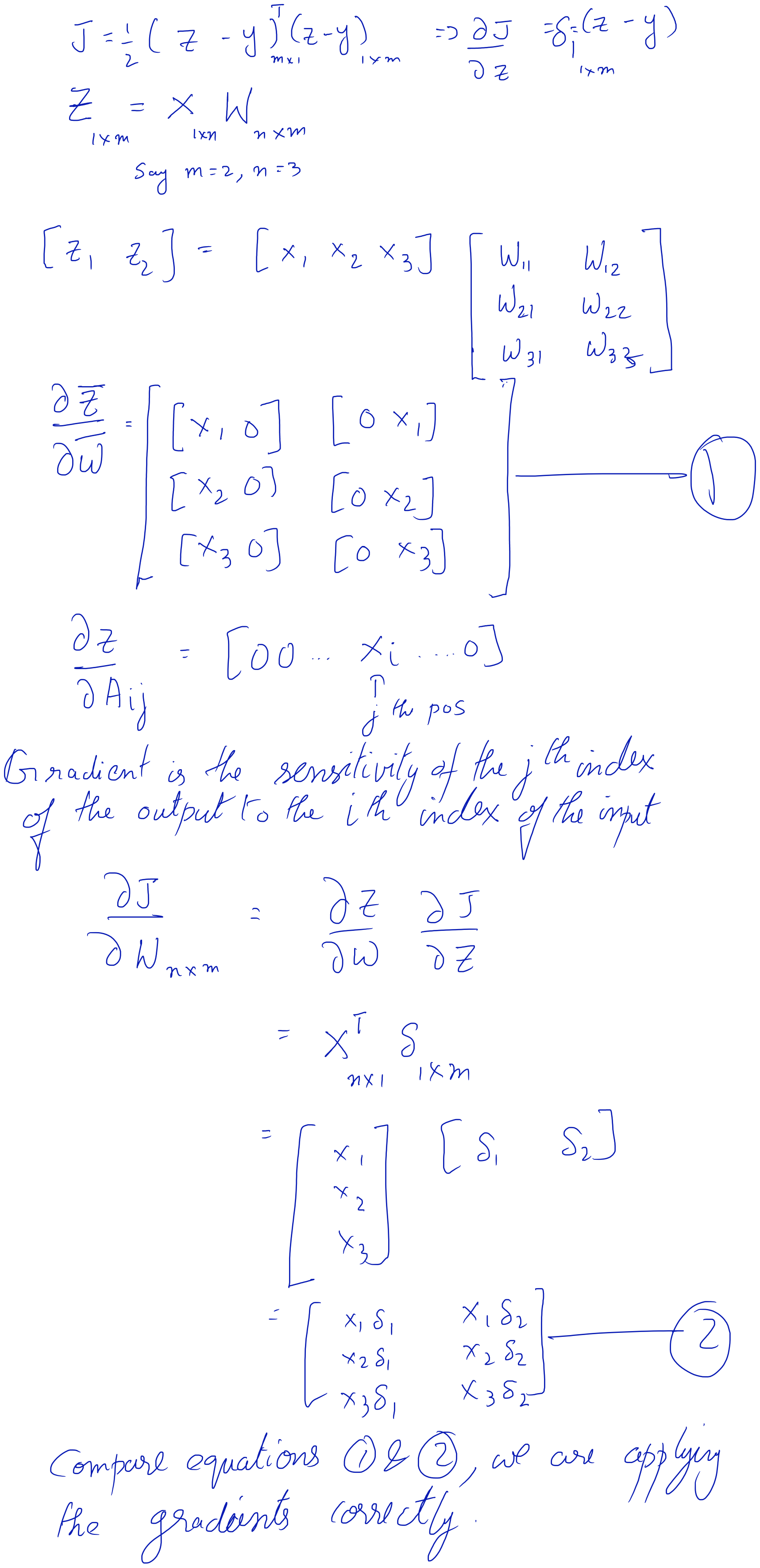
Learnings from implementing gradient

Tried to gradient descent through \(\exp\left(\frac{-2x^2 + y^2 -xy}{2}\right)\). A trick that worked well was to scale the step size by the inverse of the norm of the gradient. Since the Gaussian reaches an asymptote quickly away from the mode, if we start the descent from afar, the gradient is essentially zero and the step sizes are extremely small, whereas close the the peak the gradient is fairly strong (large). Scaling the step size by the inverse of the gradnorm, helps move quicker.

This works here as the gradients are derived analytically with little noise (only from floating pt precision). If we were to do this with an objective function approximated from data, inverse scaling with the grad norm with high variance, can throw us off track.

import numpy as np
from numpy import linalg

def f(x, y):
    return np.exp(-(2*x*x + y*y - x*y) / 2)

def gradf(xy):
    x, y = xy
    return np.array(
        [
            1/2 * (-4*x + y) * f(x, y),
            1/2 * (x - 2*y) * f(x, y)
        ],
    )

#########################
# Gradient descent
X = np.array([1, 1])
# History of gradient descent points.
GDX = np.zeros((100, 2))
i = 0
while i< 100_000:
    J = gradf(X)
    # NOTE: the inverse of the grad norm, helped move out of plateaus when beginning
    # from afar.
    X = X + 0.0001 / linalg.norm(J) * gradf(X)
    if i%1000 == 0:
        GDX[i//1000,:] = X
    i+= 1

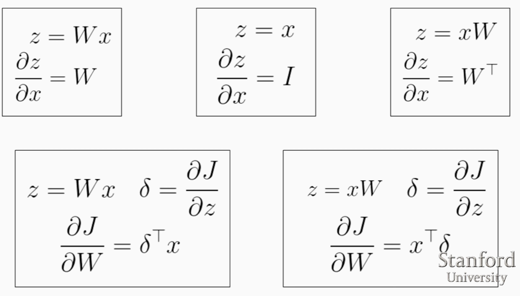
Gradient CheatSheet

Watch 20mins of this lecture.

Gradient of scalar by vector

Gradient of vector by vector

Gradient of scalar by matrix

Gradient of vector by matrix

Advanced optimisation techniques

Given some loss function \(J(\theta)\) and gradient \(\nabla_{\theta} J(\theta)\), we can use more advanced optimisation algorithms than canonical gradient descent ie.,

Some of these algorithms are LBFGS, BFGS and conjugate gradient descent. Some advantage include their ability to arrive at a reasonable learning rate themselves, usually a different one each time. This could be arrived at through the Line Search algorithm. They often converge faster than gradient descent.

Convex optimisation

Credits for the images below: Visually Explained youtube channel.
Youtube video series.

Optimisation

Decision variable: \(x \in \mathcal{R}^n\)

Cost function: \(f:\mathcal{R}^n \rightarrow \mathcal{R}\)

Constraints

• Equality constraints
  \(h(x)=0, i=1,...\)
  Example: \(x_1+x_2+...= 0\)

• Inequality constraints
  \(g(x) \leq 0 j=1, \dots\)
  Example: \(x_1^2 + x_2^2 \leq x_3^2\)

The constraints, together form the feasible set.

Examples

Linear program

When the cost function \(f(x)\), the equality constraints \(h(x),\) and the inequality constraints \(g(x)\) are all linear, the problem is called a linear programming problem.

To visualise linear functions \(f(x) = c^T x + d\), either as a hyperplane or a normal vector.

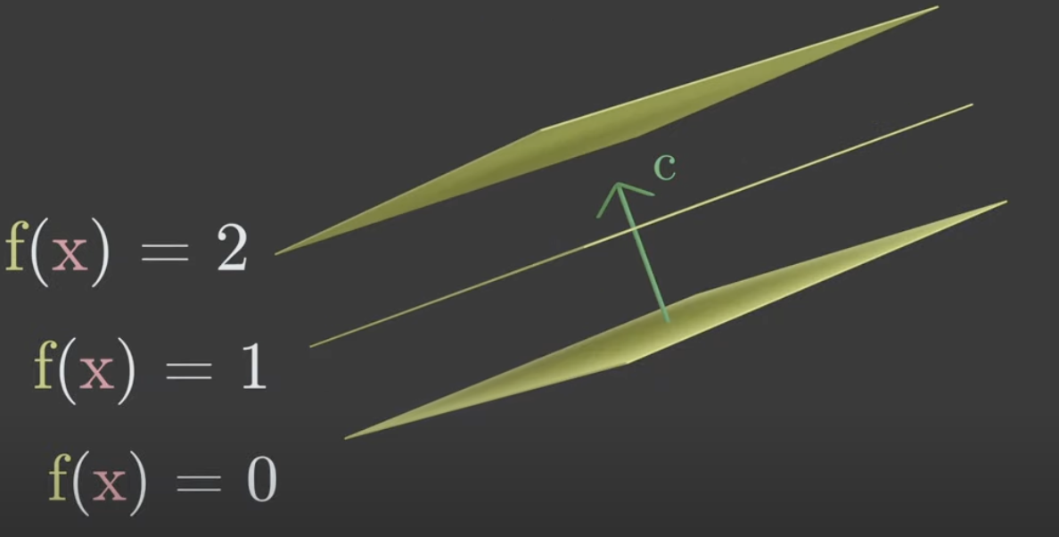
Hyperplane

Think of a hyperplane as planes \(f(x)=0, f(x) =1, f(x) =2 ....\).

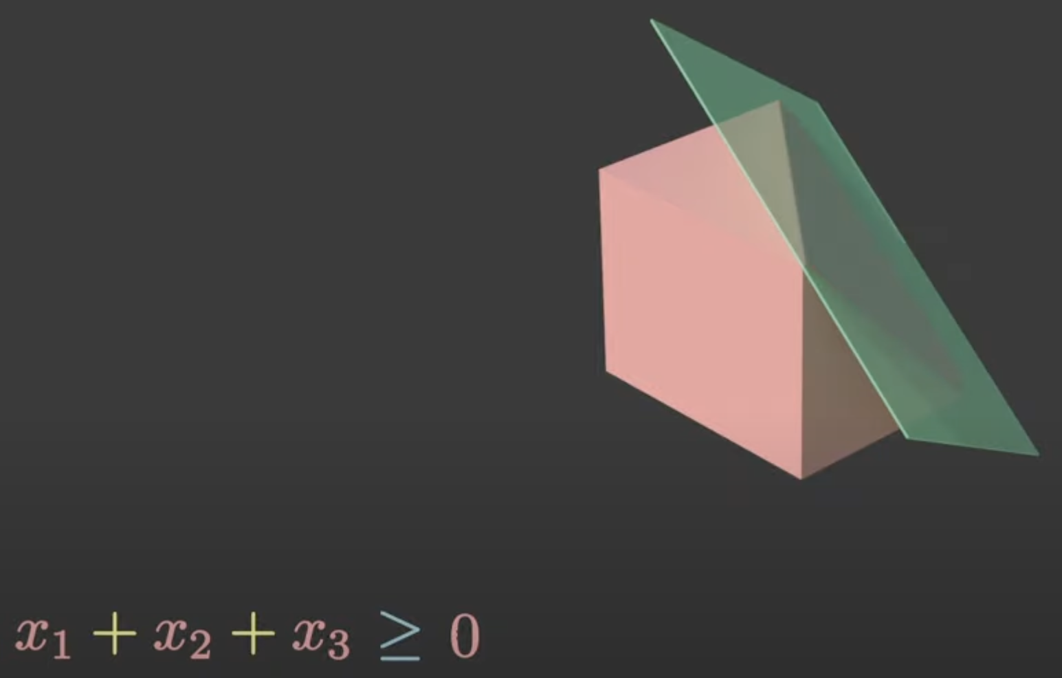
Hyperplane divides a space into three regions. The positive half space \(x_1+x_2+x_3>0\), null region or the hyperplane itself \(x_1+x_2+x_3=0\) and the negative half space \(x_1+x_2+x_3<0\). A linear inequality constraint will cut off a part of the feasible space.

Linear regression

In linear regression, we have no constraints but our cost function is simply \(|| \mathbf{Ax} - \mathbf{b}||^2\), is a quadratic loss function.

Portfolio optimisation

You are given a list of assets like stocks. Goal to find which assets to buy and have finite budget (decision variable). You have to maximise profit (cost function). Constraints could be total budget and maximum volatility.

Convexity

Three types of convexity

• Sets: A set is convex, all values between to elements of the set exist in the set. Imagine a set a blob with a hole in it.
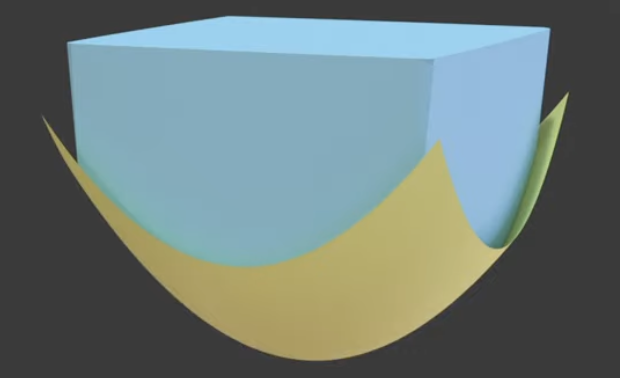
• Function: It’s epigraph, the region of the space above the function is convex.

• Optimisation: The cost function, \(f(x)\) is convex. The inequality constraints are convex \(g_i(x) \leq 0, \forall i\) and the equality constraint is linear, \(h_j(x)=0, \forall j\). The equality is linear because it can be written as two convex functions, \(h_j \leq 0\) and \(h_j \geq 0\) and this can only occur for a linear \(h_j(x)\).

Duality

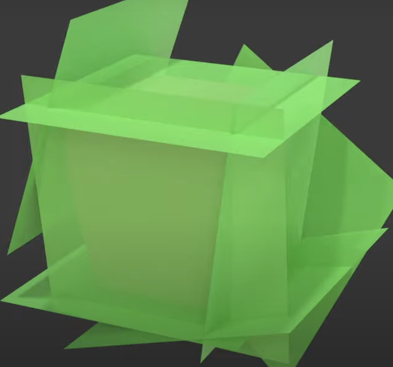
• Sets: The definition above is internal. We can have an external definition. Take a hyperplane that supports this set (the set falls on the positive regions of the hyperplane). A convex set is such that if you take the intersection of the positive regions of all the support hyperplane you recover the convex set. There can be infinitely many linear inequalities (hyperplane). Imagine defining a circle, we need infinite tangents.

• Functions: Duality let’s you extrapolate the local behaviour of a function to the global behaviour of the function. \(f(x)\) is convex iff, if it’s graph is always above it’s tangent hyperplanes for all values of x.

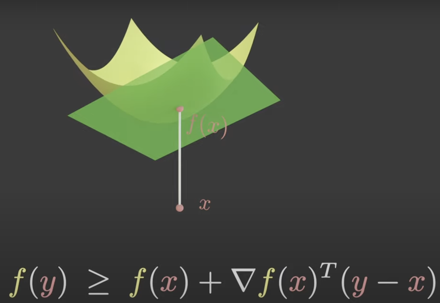
If you find the value where \(\nabla f(x) = 0\), then it absolutely is global minima as it’s a flat hyperplane and all values of \(f(x)\) need to be greater than this value. Using this property we can solve the minimum of an uncontrained optimisation of convex functions by taking the gradient and setting it to 0.

We went from a gradient at a local point to a global property of this function.