NN Activations & Normalisation Layers

Activation functions
1. Favourable properties of an activation function
2. Pros & cons of different functions
Normalisation layers

A concise peek into NN activation functions and normalisation routines.

Activation functions

Sigmoidal functions: Sigmoid and tanh
ReLu and friends: ReLu, Leaky-ReLu, PReLu, ELU.
From CMU archives.

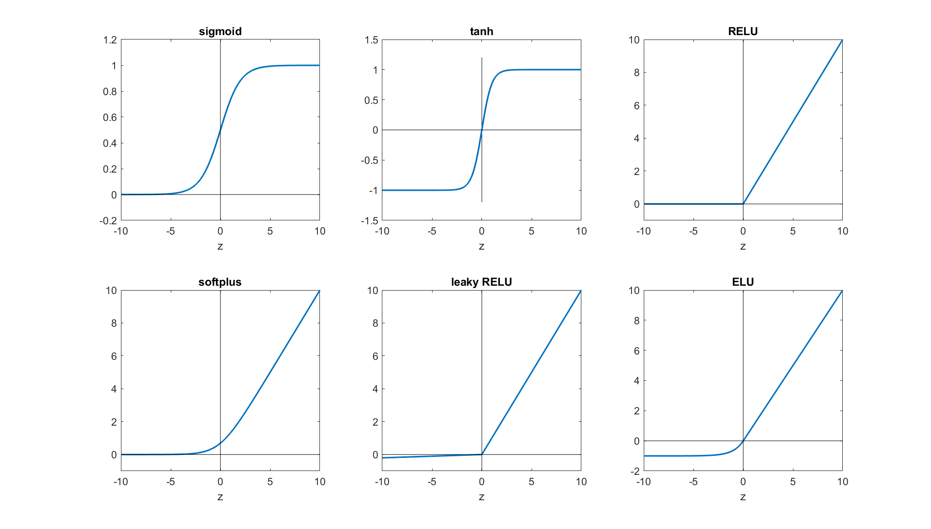
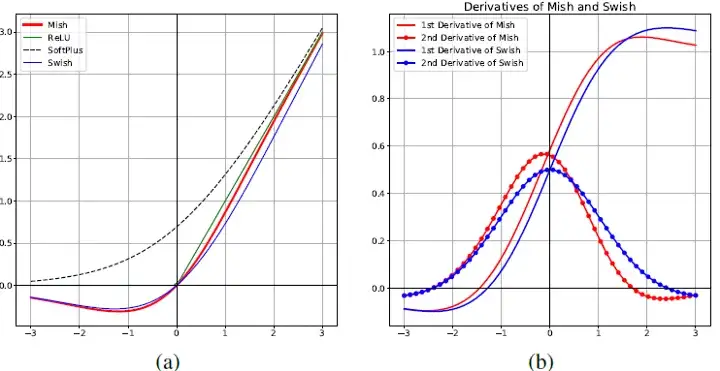
Smoothed ReLu-like: Softplus \(\left\{\log(1 + \exp x)\right\}\), Swish \(\left\{ x \sigma(x) = \frac{x}{1+\exp(-x)} \right\}\), Mish \(\left\{ x \tanh(\text{softplus}) \right\}\)
From medium

Favourable properties of an activation function

Unbounded: tanh, sigmoid are squashing functions whereas ReLu-like activations are unbounded. Though ReLu does cut off half of the input. Squashing functions tend to squash gradients and can lead to vanishing gradient issues.
Dead neuron: While randomly initialising weights, we could initialise extreme weight values such that tanh is saturated or ReLu input is negative for all input training instances. In those scenarios, the neuron never receives gradients and never learns. ReLu is prone to this issue.
Zero centeredness: Zero centeredness appears to be advantageous for backpropagation training. ReLu and sigmoid are not zero centered whereas tanh is. Having said that ReLu outperforms tanh for very deep networks in practice.
Differentiable: ReLu, Leaky-ReLu and PReLu are not differentiable at 0.
Fast to compute (no exponentiation).

Pros & cons of different functions

After the step function, sigmoid was one of the earliest activation function. However it suffers from saturation and not being zero-centered.
tanh is preferred over sigmoid as it is zero centered.
ReLu allows gradients to flow freely in the positive domain. However, it can be prone to dead neurons. Besides, it is not zero-centered. It does work well in practice for deep nets.
Leaky-ReLu essentially provides a small slope for negative values, whereas PReLu let’s backprop learn the slope. This is designed to allow gradients to still flow for negative input values, preventing dead neurons. Though in practice they don’t perform significantly better than ReLus.
ELU again avoids the gradient blocking at the negative domain unlike ReLu. However it’s also differentiable at 0 and smoothly converges to 0 for very low values of inputs.
Swish and Mish are non monotonic activation functions that seem to outperform other activation functions in recent time. They allow somewhat large gradients for small negative values of inputs and then asymptote out to zero for very negative inputs.

Normalisation layers

Layers discussed below:

Batch normalisation
Layer normalisation
Instance normalisation
Group normalisation

Resources: medium, nptel lectures.

For CNN discussions below consider the training batch consisting of a 4-D tensor of dimensions \(N \times C \times H \times W\). \(N\) is the batch size (images), \(C\) is the number of convolution channels at this depth, \(H \times W\) are the spatial dimensions of the image.

Batch normalisation

Applied to linear layers and CNN.

Linear layer: Consider a \(N \times D\) training batch matrix, with \(N\) data points and \(D\) features. We standardise each feature by computing it’s mean and standard deviation. We keep track of \(D\) \(\mu\)s and \(\sigma^2\)s.

ε = 1e-5
X = torch.randn(10, 4)
μ = X.mean(dim=0, keepdims=True)  # 1 x 4
ν = X.var(dim=0, keepdims=True)  # 1 x 4
Xstd = (X - μ) / (ν + ε)**(0.5)  # 10 x 4
Xbn = ɣ * Xstd + β  # ɣ, β -> 1 x 4; scale and shift

CNN: For CNN’s we compute one mean and standard devation per channel. We will have \(C\), \(\mu\)s and \(\sigma\)s.

ε = 1e-5
X = torch.randn(10, 4, 128, 64)  # 10 imgs, 4 channels, H - 128, W - 64
μ = X.mean(dim=[0,2,3], keepdims=True)  # shape [1, 4, 1, 1]
ν = X.var(dim=[0,2,3], keepdims=True)  # shape [1, 4, 1, 1]
Xstd = (X - μ) / (ν + ε)**(0.5)  # 10 x 4 x 128 x 64
Xbn = ɣ * Xstd + β  # ɣ, β -> [1, 4, 128, 64]; scale and shift

Salient points

The fact that the forward pass depends on other samples in the batch has a regularising effect (entropy is good in training).
It outperforms other normalisation techniques.
Batch norm couples examples and often leads to bugs. Batch norm needs to keep track of the training mean and stddev for each feature. So we need to switch between train and eval phases while using batch norms.
Batch norm requires the batch size to not be very small (rule of thumb > 16). This is a hinderance to distributed training.
Batch norm cannot be easily applied to RNNs as we need a different batch norm layer for each time step.

Layer normalisation

Applied to linear, CNN, and RNN layers.

Linear layer: Consider a \(N \times D\) training batch matrix, with \(N\) data points and \(D\) features. We standardise all the features of a single training/test instance with a single \(mu\) and \(sigma\) learnt from all the features of that instance. We compute \(N\) \(\mu\)s and \(\sigma^2\)s but we don’t have to keep track of them during testing.

ε = 1e-5
X = torch.randn(10, 4)
μ = X.mean(dim=1, keepdims=True)  # 10 x 1
ν = X.var(dim=1, keepdims=True)  # 10 x 1
Xstd = (X - μ) / (ν + ε)**(0.5)  # 10 x 4
Xln = ɣ * Xstd + β  # ɣ, β -> 1 x 4; scale and shift

CNN: For CNN’s we compute one mean and standard devation per image across all channels. We would have computed \(N\), \(\mu\)s and \(\sigma\)s.

ε = 1e-5
X = torch.randn(10, 4, 128, 64)  # 10 imgs, 4 channels, H - 128, W - 64
μ = X.mean(dim=[1,2,3], keepdims=True)  # shape [10, 1, 1, 1]
ν = X.var(dim=[1,2,3], keepdims=True)  # shape [10, 1, 1, 1]
Xstd = (X - μ) / (ν + ε)**(0.5)  # 10 x 4 x 128 x 64
Xbn = ɣ * Xstd + β  # ɣ, β -> 4 x 128 x 64; scale and shift

For RNN’s we don’t normalise over the time dimension unlike CNN.

Instance normalisation

Applied to CNN layers. Not applicable to training data tensors smaller than 3 dimensions.

CNN: For CNN’s we compute one mean and standard devation per image per channel. We will have \(N \times C\), \(\mu\)s and \(\sigma\)s.

ε = 1e-5
X = torch.randn(10, 4, 128, 64)  # 10 imgs, 4 channels, H - 128, W - 64
μ = X.mean(dim=[2,3], keepdims=True)  # shape [10, 4, 1, 1]
ν = X.var(dim=[2,3], keepdims=True)  # shape [10, 4, 1, 1]
Xstd = (X - μ) / (ν + ε)**(0.5)  # 10 x 4 x 128 x 64
ɣ = β = torch.randn(1, 1, 128, 64)
Xin = ɣ * Xstd + β  # ɣ, β -> 1 x 1 x 128 x 64; scale and shift

Group normalisation