Random variable
Given an input space U, X is a random variable that maps every element in U to a real number \(\mathcal{R}\), i.e., \(X:U \rightarrow V\).
Say \(U\) is a set of all 3 digit binary numbers viz., \(U=\{000, 001, 010, 011, 100, 101, 110, 111\}\) and X maps element to the last digit (lsb=least significant bit). Hence, \(V= \{0, 1\}\). The probability of \(P(X=0) = 0.5\) and \(P(X=1) = 0.5\). Half the numbers map to \(1\) and other to \(0\). Now the probability of \(P(X=0)\) is the same as the probability of sampling a number in the input space \(U\), that will cause \(X\) to map to \(0\). Here we are implicitly assuming that the probability of sampling any element in \(U\) is the same or elements in \(U\) are distributed uniformly.
Independence
If X and Y are two independent random variable. Then \(P(X=x,Y=y) = P(X=x)P(Y=y)\), that is knowing that \(X\) takes the value \(x\), tells you nothing about what value \(Y\) will take and vice-versa.
Let’s say X and Y are binary variables i.e., \(X:U\rightarrow \{0,1\}\) and \(Y:U \rightarrow \{0,1\}\). In order to formally prove \(X\) and \(Y\) are independent, we will have to prove that the joint \(P(X=0, Y=0) = P(X=0)P(Y=0), P(X=0,Y=1) = P(X=0)P(Y=1)...\) for all 4 possibilities.
Linearity of expectations
Let \(X_1, X_2, \cdots, X_n\) be random variables defined in the same sample space, then
\[E\left[\sum_{j=1}^n X_j\right] = \sum_{j=1}^n E[X_j]\]Linearity expecations works even if the random variables are not independent. This is certainly not true for products of random variables.
Gaussian or Normal distribution
Univariate
\[\mathcal{N}(x;\mu, \sigma) = \frac{1}{\sigma \sqrt{2 \pi}} \exp\left(\frac{-(x-\mu)^2}{2\sigma^2}\right)\]Multivariate
\[\mathcal{N}(\mathbf{x};\mathbf{\mu}, \Sigma) = \frac{1}{ ({2 \pi})^{\frac{d}{2}} \sqrt{|\Sigma|}} \exp\left\{\frac{-1}{2}(\mathbf{x}-\mathbf{\mu})^T \Sigma^{-1} (\mathbf{x}-\mathbf{\mu}) \right\}\]where \(x \in R^d, \mu \in R^d, \Sigma \in R^{d\times d}\)
\[\mu = \frac{1}{m} \sum_{i=1}^m \mathbf{x_i}\] \[\Sigma = (\mathbf{x}-\mathbf{\mu}) (\mathbf{x}-\mathbf{\mu})^T\]If \(X\) is \(n \times d\), then
\[\Sigma = \frac{(\mathbf{X}-\mathbf{\mu})^T (\mathbf{X}-\mathbf{\mu})}{n-1}\]Poisson distribution
This is used to model number of events in a given time period. The events occur randomly at a constant rate. It is a discrete probability distributions, the number of events are always non-negative integers.
Examples:
- Number of clicks on a website between 10pm-12pm.
- Number of road accidents in a city between 8am-9am.
- Number of people in a queue for a restaurant between 6pm-9pm.
Modelled as
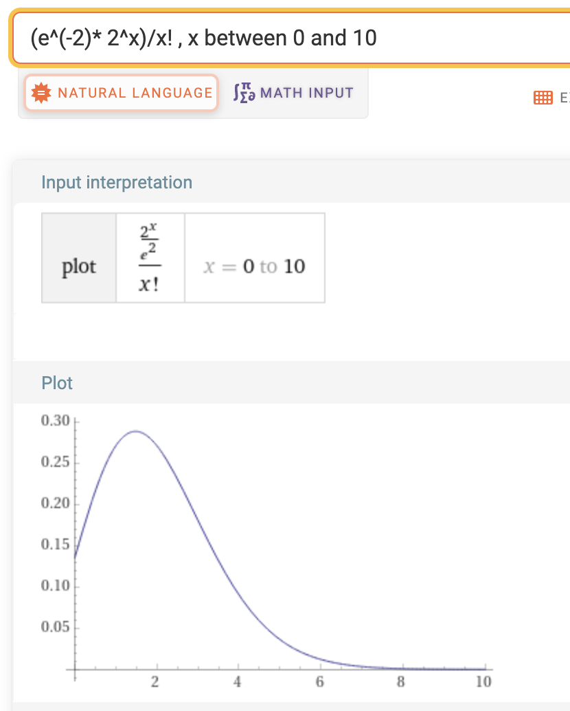
\[P(x=x_i) = \dfrac{e^{-\lambda} \lambda^{x_i}}{x_i!}\]where \(\lambda\) is the mean number of events in that time period. As \(x\) increases, both the numerator and the denominator grows exponentially. However the denominator (factorial) first grows slowly and then grows extremely fast and ends up squashing the numerator leading the value to asymptotically vanish to 0.
See wiki for examples of computing the probabilities with the poisson distribution.
From Wiki: The Poisson distribution is also the limit of a binomial distribution, for which the probability of success for each trial equals \(\lambda\) divided by the number of trials, as the number of trials approaches infinity.
From Wolfram:
ML Measures and Metrics
Mutual information
MI of two random variables measures how much knowing one random variable reduces the uncertainty of the other random variable. If the RV are independant, then MI is 0 and if knowing one fully determines the other MI is 1. It’s defined as
\[MI(X_1, X_2) = \sum_{x_i}\sum_{x_j} P(X_1=x_i, X_2=x_j) \log \frac{P(X_1=x_i, X_2=x_j)} {P(X_1=x_i) P(X_2=x_j)}\]The above can also be thought of as the KL-Divergence loss from approximating the joint of \(X_1\) and \(X_2\) with the marginals.
Substituting the joint as the product of the marginals \(P(X_1, X_2) = P(X_1) P(X_2)\), it’s easy to see how MI will be 0 for independent RV.
Correlation coefficient
Correlation coefficient \(\rho_{xy}\) is a measure of the strength of the linear relationship of two RV. Highest correlation is at \(\rho_{xy} = \pm 1\) and when two RV are linearly uncorrelated \(\rho_{xy} = 0\).
\[\text{Pearson correlation cofficient} = \rho_{xy} = \frac{cov(x, y)}{\sigma_x \sigma_y}\]