Table of Contents
Graph representation
Credits: Some of the images here are taken from the Design of algorithms course from Stanford.
Elements: Nodes or vertices \((V)\) and edges \((E)\).
Types
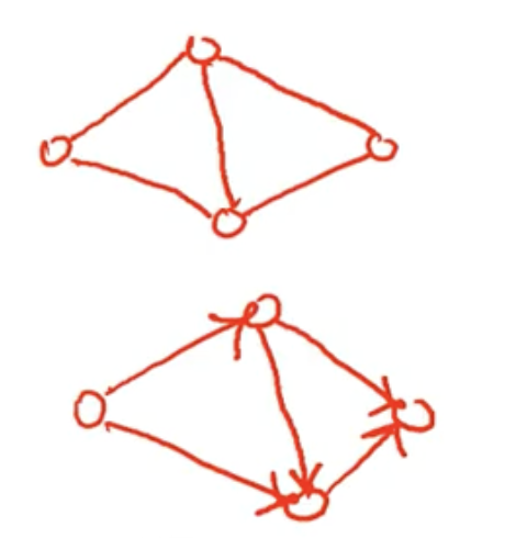
Edges are directed or undirected
- Undirected graph - The nodes are unordered.
- Directed graph - Has directed edges. There is a first (tail) and the last vertex (head) or end point. Directed edge is also called an Arc. If a -> b, then a is the tail and b is the head.
Terminologies
- Parallel edges: They are edges connecting the same two nodes.
- Connected graph: There is a path between any pair of vertices.
- Complete graph: A graph with all nodes connected to each other.
- Degree of a node: Number of egdes incident on the node.
Facts
- Number of edges: n-num vertices and m-num edges. For a connected undirected graph and with no parallel edges, the min and max number of possible edges is \((n-1)\) and \(\frac{n(n-1)}{2}\).
- Sparse graph vs Dense graph: m is \(\Omega(n)\) and \(O(n^2)\). If m is closer to \(\Omega(n)\) then it’s a sparse graph, if it’s closer to \(\Omega(n)\) it’s a dense graph.
- \(\sum_v degree(v) = 2m\). Each edge is a part of two nodes.
Adjacency matrix
For a graph with n-vertices, the adjacency matrix is a \(n\times n\) matrix, where each entry A[i,j] represents if there is an edge btw the two nodes i and j.
Extensions
- Parallel edges: A[i,j] has number of edges.
- Weighted edges: A[i,j] has weights.
- Directed edges: A[i,j], 1 if from i to j and -1 if from j to i.
Space complexity: O(n^2). Can beat this with sparse matrix representations.
Adjacency list
We store the following datastructure
Programming interview style
- Nodes are all integers from
0ton-1, we use alist[set[int]]. Each item in the list is a node and each element in the set are the nodes at the head of the outward arc from this node. If undirected it’s simply the neighbour of this node. - Node are node datatype. We use
dict[Node,set[Node]]. It’s similar to the above and of course we need to make the node hashable.
def _build_graph(edges: list[list[int]], num_nodes: int) -> list[set]:
    """Builds a adjacency-list type graph from a list of edges.
    :param edges: Each item is an edge [i, j] such that we have an edge i -> j.

    Sample input::
        edges=[[1,0], [2,0], [3,2], [1,3]], num_nodes=5
        [1] -> [0]   [4]
         |      ^
         v      |
        [3] -> [2]

    Sample output::
        graph=[set(), {0,3}, {0}, {2}, set()]
    """
    adj_set = [set() for _ in range(num_nodes)]
    for tail, head in edges:
        adj_set[tail].add(head)
    print(f"{adj_set=}")
    return adj_set
Production style
Undirected
@dataclass
class Edge:
    nodes: tuple['Node', 'Node']

@dataclass
class Node:
    val: int = 0
    edges: Optional[set['Edge']] = None

"""
Graph
        (0) -- (1)
         |
        (2)
"""
nodes = [Node(val=0), Node(val=1), Node(val=2)]
edges = [Edge(nodes=(nodes[0], nodes[1])), Edge(nodes=(node[0], node[2]))]
nodes[0].edges = [edge[0], edge[1]]
nodes[1].edges = [edge[0]]
nodes[2].edges = [edge[1]]
Directed
@dataclass
class Edge:
    tail: 'Node'
    head: 'Node'

@dataclass
class Node:
    val: int = 0
    outward_edges: Optional[set['Edge']] = None
    # This variable is optional and adds to storage. We
    # can get away with just the outward edges.
    inward_edges: Optional[set['Edge']] = None

"""
Graph
        (0) --> (1)
         Ʌ
         |
        (2)
"""
nodes = [Node(val=0), Node(val=1), Node[val=2]]
edges = [
    Edge(tail=nodes[0], head=nodes[1]),
    Edge(tail=nodes[2], head=nodes[0]),
]
nodes[0].outward_edges = {edges[0]}
nodes[0].inward_edges = {edges[1]}
nodes[1].outward_edges = {}
nodes[1].inward_edges = {edges[0]}
nodes[2].outward_edges = {edges[1]}
nodes[2].inward_edges = {edges[0]}
Space complexity: \(\theta(m+n)\). This can be \(O(n^2)\) for a compelte graph. However, this is an overestimate. The above complexity handles this as \(m\) will be \(n^2\), in this case.
Which one should you choose
Depends on graph density and operations we want to support.
- For low density, high number of nodes in a graph, it’s more efficient to choose adjacency list. Imagine the internet where the number of webpages is extremely large and the graph is rather sparse.
- For graph search, adjacency list provides the appropriate operations we need.
Graph Algorithms
Topological sort
Algorithm that given a directed acyclic graph, returns an ordering of the nodes with the following property:
For any two nodes in the output array TS with indices i and j such i < j, then
all outward arcs from TS[j] will end in a node TS[k] such that k > i.
The only condition for a Topological Sort to exist is that the directed graph needs to be acyclic.
Algorithm
The algorithm piggybacks on DFS.
- Wrapper function and a DFS helper function.
- In wrapper function, create
- create an output list with the same length as number of nodes (n).
- create a seen hashset.
- Initialise a global index to n-1.
- Iterate over all the nodes to handle disjoint nodes.
- In the dfs helper function
- mark the node as seen
- recurse over adjacent nodes.
- At the end of the recursion, add the node to the current index and decrement the index.
import typing
from dataclasses import dataclass
# Graph represented as an adjacency list, `len(graph)` is num nodes and
# `len(graph[i])` is number of adjacent numbers from node `i`.
Graph = typing.NewType('Graph', list[list[int]])

@dataclass
class Index:
    ix: int

def topsort(graph: Graph) -> list[int]:
    if not graph:
        return []
    n = len(graph)
    output, output_ix, seen = [None]*n,  Index(ix=n-1), set()
    for i in range(n):
        if i in seen:
            continue
        _dfs(graph=graph, node=i, seen=seen, output=output, output_ix=output_ix)
    return output

def _dfs(
    graph: Graph, node: int, seen: set[int], output: list[int], output_ix: Index,
) -> None:
    seen.add(node)
    # This will be only be empty for the sink node; equally this loop will be a no-op
    # if all the descendents have already been visitied
    for adj in graph[node]:
        if adj in seen:
            continue
        _dfs(graph=graph, node=adj, seen=seen, output=output, output_ix=output_ix)
    output[output_ix.ix] = node
    output_ix.ix -= 1

#          ┌────┐
#   ┌──────► 1  ├───────┐
#   │      └────┘       │
# ┌─┴──┐             ┌──▼─┐
# │ 0  │             │ 3  │
# └─┬──┘             └──▲─┘
#   │      ┌────┐       │
#   └──────► 2  ├───────┘
#          └────┘
print(topsort(graph=Graph([[1,2],[3], [3], []])))
Cycles in graphs
Cycles in Directed Graphs
A directed graph with no cycles is called a DAG or a Directed Acyclic graph.
Algorithm
The algorithm uses DFS and 3 sets, explore, visiting and done.
- We add all the nodes to the
exploreset. - In the outer wrapper method, while loop until
exploreis not empty, call the_dfshelper method on any node inexplore. - In
_dfshelper- we move
nodefromexploretovisiting - we iterate over
neighbours of
node. - If the neighbour is in
done, we continue - If it’s in
visitingthat is we were able to reach this neighbour earlier in the recursion stack we have found a cycle, immediately returnTrue. - Otherwise we visit the neighbour. If the neighbour returns
True, we immediately returnTrue. - If none of the neighbours have seen a cycle, then we simple move this
nodeto thedoneset and returnFalse.
- we move
def has_dag_cycle(graph: list[set]) -> bool:
    """Checks if a DAG has a cycle.

    :param graph: Each item in a list is a node and each element in the set are the
        nodes at the head of the outward arc from this node.

    Sample cyclic input::
        [{2}, {0}, {3}, {1}]

        [1] ->  [0]
         ^       |
         |       v
        [3] <-  [2]

    Sample non-cyclic input::
        [{}, {0,3}, {0}, {2}, {}]
          0    1     2    3    4

        [1] -> [0]     [4]
        |       ^
        v       |
        [3] -> [2]
    """
    explore = set(range(len(graph)))
    visiting, done = set(), set()
    while explore:
        if _cycle_dfs(
            node=next(iter(explore)),
            graph=graph,
            explore=explore,
            visiting=visiting,
            done=done,
        ):
            return True
    else:
        return False

def _cycle_dfs(node, graph, explore, visiting, done):
    _move_node(node, explore, visiting)
    for adj in graph[node]:
        if adj in done:
            continue
        if adj in visiting:
            # Found a cycle. This node was visited earlier while recursing to this node.
            # `adj` is both an ancestor and and a descendent of the current node.
            return True
        if _cycle_dfs(
            node=adj, graph=graph, explore=explore, visiting=visiting, done=done,
        ):
            return True
    else:
        _move_node(node, visiting, done)
        return False

def _move_node(node, from_set, to_set) -> None:
    """Side effect, mutates the input sets"""
    from_set.discard(node)
    to_set.add(node)
Cycles in Undirected Graphs
Two algorithms DFS and using Disjoint Set Union (DSU).
See a notebook version of the code below with graph visualisations on nbviewer.
Graphs tested below
See blog on visualising graphsAcyclic graph
Cyclic graph
DSU: We initialise the DSU with singleton sets containing each graph node. We
iterate over edges. Gotcha: for an edge a-b, if this edge appears twice once for
a and once for b, we ensure we only iterate over it once. We check if the nodes
of the edge are already connected which means we have a cycle, otherwise we simply
union the two nodes. Time and memory complexity is \(O(V)\). We iterate over the edges
but if there’s more edges than nodes, then we definitely have a cycle.
from collections.abc import Iterable
from dataclasses import dataclass
from dataclasses import field
from typing import Generator
from typing import Hashable

@dataclass
class DSU:
    """Disjoint Set Union implementation."""

    parent: dict[Hashable, Hashable] = field(default_factory=dict)
    rank: dict[Hashable, int] = field(default_factory=dict)

    def add_nodes(self, ns: Iterable[Hashable]) -> 'DSU':
        for n in ns:
            self.add_node(n=n)
        return self

    def add_node(self, n: Hashable) -> 'DSU':
        self.parent[n] = n
        self.rank[n] = 1
        return self

    def find_leader(self, n: Hashable) -> Hashable:
        if self.parent[n] == n:
            return n
        self.parent[n] = self.find_leader(n=self.parent[n])
        return self.parent[n]

    def union(self, n1: Hashable, n2: Hashable) -> 'DSU':
        n1_leader = self.find_leader(n=n1)
        n2_leader = self.find_leader(n=n2)
        if n1_leader == n2_leader:
            return
        if self.rank[n1_leader] > self.rank[n2_leader]:
            self.parent[n2_leader] = n1_leader
        elif self.rank[n1_leader] < self.rank[n2_leader]:
            self.parent[n1_leader] = n2_leader
        else:
            # equal ht trees
            self.parent[n2_leader] = n1_leader
            self.rank[n1_leader] += 1
        return self

    def is_connected(self, n1: Hashable, n2: Hashable) -> bool:
        return self.find_leader(n=n1) == self.find_leader(n=n2)

def has_undirected_cycle(graph: dict[str, set[str]]) -> bool:
    """Finds cycles in an undirected graph.

    :param graph: The keys of the dict are the graph nodes which are strings. The set
        of strings they hold are the set of nodes connected to them.
    """
    dsu = DSU()
    dsu.add_nodes(ns=graph.keys())
    for n1, n2 in _iter_edges(graph):
        if dsu.is_connected(n1, n2):
            return True
        dsu.union(n1, n2)
    else:
        return False

def _iter_edges(graph: dict[str, set[str]]) -> Generator[tuple, None, None]:
    """Iterate through edges in a undirected graph. In an undirected graph, two
    connected nodes A and B will have each other in their edge set and hence the edge
    appears twice, we have to ensure we only yield an edge once.
    """
    seen = set()
    for n, adjs in graph.items():
        for adj in adjs:
            edge = tuple(sorted([n, adj]))
            if edge in seen:
                continue
            seen.add(edge)
            yield edge

# [d-a-c] [f] [b-e]
graph = {'a': {'c', 'd'}, 'b': {'e'}, 'c': {'a'}, 'd': {'a'}, 'e': {'b'}, 'f': {}}
has_undirected_cycle(graph)
# False

# [f]
#
#  b - a - c
#  | /  \
#  e     d
graph = {
    'a': {'c', 'd', 'e', 'b'}, 'b': {'e', 'a'}, 'c': {'a'},
    'd': {'a'}, 'e': {'b', 'a'}, 'f': {}
}
has_undirected_cycle(graph)
# True
DFS: Simply DFS keeping track of the seen set, if you ever see a node again besides the node you can from, you have a cycle. It’s easy to understand by visualising an undirected graph with no cycles (a connected acyclic graph is a tree). Time and memory complexity is \(O(V)\)
def has_undirected_cycle_dfs(graph: dict[str, set[str]]) -> bool:
    seen = set()
    # The graph may not be fully connected, we need to DFS through each connected set.
    for n in graph:
        if n in seen:
            continue
        if _ucycle_dfs(graph=graph, node=n, parent=None, seen=seen):
            return True
    else:
        return False

def _ucycle_dfs(
        graph: dict[str, set[str]], node: str, parent=Optional[str], seen: set) -> bool:
    seen.add(node)
    for adj in graph[node]:
        if adj == parent:
            continue
        elif adj in seen:
            # We have reached neighbour before through different path, this is a cycle.
            return False
        elif _ucycle_dfs(graph=graph, node=adj, parent=node, seen=seen):
            return False
    else:
        return True
Find all shortest paths between two nodes
The workhorse of this algorithm will be BFS.
Algorithm
- We need 3 functions, a wrapper, a bfs and finally a
trace_path. - The wrapper will pass into bfs,
graph,src. Bfs will returnparents. - BFS, will maintain two additional maps,
distsandparents.distsis the shortest distance to each node from source.dists[src] = 0.parentscontains a set of parents which result in the same shortest distance to this node from the source.parents[src] = None.
- The queue in BFS will begin with
src. We while over q, pop the left node and iterate over adjacent nodes. If the shortest distance of adjacent node is- greater than
dists[node] + 1, then we have a brand new shortest path and we need to re-explore it’s neighbours so that we can update their paths, so we need to add it to the queue. - equal to
dists[node] + 1, then we just add it to parents (no need to update neighbours). - lesser than
dists[node] + 1, then we do nothing and move on.
- greater than
trace_pathwill be called withparents,end,path=[],paths=[]. We will begin at theendnode and we recursively calltrace_pathfor every parent until we reachparent=Noneforsrcand we add thepathto paths after reversing it. After iterating over all the parents we removeendfrom path.
Takeaway: For path finding problems, keep track of parents in a dict or list and then trace path in a separate function.
Code
import collections
from typing import NewType
from typing import Optional

#: A map of node name to it's set of adjacent nodes.
Graph = NewType('Graph', dict[str, set[str]])
#: A path described by a list of node names.
Path = list[str]

def find_shortest_paths(graph: Graph, src: str, end: str) -> list[Path]:
    """Finds all the paths with the shortest distance between src and end.

    See tests below for sample input and output.
    """
    parents = _find_min_path_parents_bfs(graph=graph, src=src)
    paths = []
    _trace_paths(end=end, parents=parents, path=Path([]), paths=paths)
    return paths

def _find_min_path_parents_bfs(graph: Graph, src: str) -> dict[str, set[Optional[str]]]:
    dists, parents = {src: 0}, {src: {None}}
    q = collections.deque([src])
    while q:
        node = q.popleft()
        for adj in graph[node]:
            adj_dist = dists.get(adj, float('inf'))
            if adj_dist > dists[node] + 1:
                # We have found a new shortest path, remove all previous parents.
                # Update adj distance and add it to the queue as we need to update it's
                # neighbours.
                dists[adj] = dists[node] + 1
                parents[adj] = {node}
                q.append(adj)
            elif adj_dist == dists[node] + 1:
                # We have found another route to adj with the shortest distance
                parents[adj].add(node)
    return parents

def _trace_paths(
    end: str,
    parents: dict[str, set[Optional[str]]],
    path: Path,
    paths: list[Path],
) -> None:
    """Side effect: populates paths."""
    if end is None:
        # We have reached the parent of source
        paths.append(list(reversed(path)))
        return
    path.append(end)
    for each_parent in parents[end]:
        _trace_paths(end=each_parent, parents=parents, path=path, paths=paths)
    path.pop()
Test
Graph we are using to test:
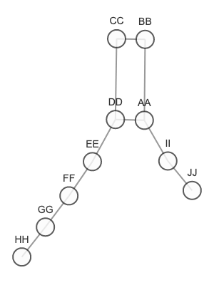
graph = {
    "AA": {"BB", "DD", "II"},
    "BB": {"AA", "CC"},
    "CC": {"BB", "DD"},
    "DD": {"AA", "CC", "EE"},
    "EE": {"DD", "FF"},
    "FF": {"EE", "GG"},
    "GG": {"FF", "HH"},
    "HH": {"GG"},
    "II": {"AA", "JJ"},
    "JJ": {"II"}
}
find_paths(graph=graph, src='BB', end='FF')
# [['BB', 'CC', 'DD', 'EE', 'FF'], ['BB', 'AA', 'DD', 'EE', 'FF']]
find_paths(graph=graph, src='BB', end='JJ')
# [['BB', 'AA', 'II', 'JJ']]
Dijkstra’s shortest path algorithm
Dijkstra’s algorithm finds the shortest path from a source node to other nodes in a weighted edge graph. If the weight was 1 for all the edges, we can simply use BFS. Dijkstra’s algorithm assumes that edges lengths are non-negative. Dijkstra’s is a Greedy algorithm. In Dijkstra’s, once a node is visited, we are guaranteed to have its shortest distance from source.
Rough sketch of the algo:
- You are given a graph and a source node.
- Instantiate
dist(dict) => node -> shortest dist from source (initially0for src and∞for the rest)parent(dict) => node -> parent_node in the shortest path (initiallyNone)visited(set) => initially empty, all the nodes visited already.heap=> Containing a tuple of (dist_from_src, node) where dist_from_src is the current shortest distance of the node from source (initially[(0, src)]).
- While the
heapis not empty andvisited.size < graph.size:
We pop nodes from the heap, and mark it as visited. We now explore the frontier, ie., all the neighbours. If the adj not in visited and the dist from source through this cur node is shorter than the previous shortest path, we update thedist[adj]andparent[adj]. We alsoheap.push((dist[adj], adj)).
Caveat: Ideally, whenever we find a shorter path for a node already in the heap, we would like to delete it from the heap and push a new tuple
(shorter_dist, node)into the heap. However, at least in python, the standard implementation doesn’t keep track of the node positions in the heap array.
We instead merely reinsert the existing node with the shorter distance, which will “bubble up” to the top of the heap. We will ignore the duplicate entry using thevisitedset check.
Time complexity: \(O(E \log V)\). Todo explain.
import heapq

def dijkstra(
    graph: dict[str, dict[str, float]],
    src: str,
    verbose: bool = False,
) -> dict:
    """Returns shortest distance and parent nodes in the shortest path from source.

    Dijkstra is very similar to BFS. Instead of a queue, we use a priority queue, where
    the priority is set by the dist from the source.

    :param graph: A map of node -> {neib: edge_wt}
    """
    dist = {
        n: float('inf') if n != src else 0.
        for n in graph
    }
    parent = {n: None for n in graph}
    heap = [(0, src)]
    visited = set()
    while heap and len(visited) < len(graph):
        _, node = heapq.heappop(heap)
        if node in visited:
            continue
        visited.add(node)
        for adj, d2adj in graph[node].items():
            if adj in visited:
                continue
            this_dist = dist[node] + d2adj
            if dist[adj] > this_dist:
                dist[adj] = this_dist
                parent[adj] = node
                heapq.heappush(heap, (this_dist, adj))
        if verbose:
            print(f"Visited{node=} \t {heap=}")
    return {"dist": dist, "parent": parent}


def get_shortest_path(graph, src, dst) -> list[str]:
    # Edge case handling
    if src == dst:
        # Same node
        return [src]
    # Edge case: not connected
    dijkstra_res = dijkstra(graph=graph, src=src)
    s2d_dist = dijkstra_res["dist"][dst]
    print(f"Distance: {s2d_dist}")
    if s2d_dist == float('inf'):
        # Not connected
        return []
    # Trace path
    parent = dijkstra_res["parent"]
    path_rev = []
    cur_node = dst
    while cur_node is not None:
        path_rev.append(cur_node)
        cur_node = parent[cur_node]
    return list(reversed(path_rev))
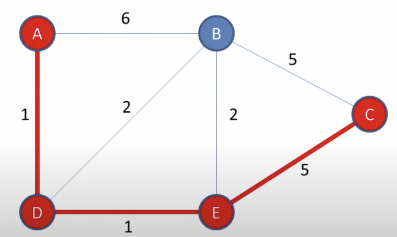
Credit for the image below https://youtu.be/pVfj6mxhdMw
# Test
graph = {
    'A': {'B': 6, 'D': 1},
    'B': {'A': 6, 'D': 2, 'E': 2},
    'C': {'B': 5, 'E': 5},
    'D': {'A': 1, 'B': 2, 'E': 1},
    'E': {'B': 2, 'D': 1, 'C': 5},
}
print(dijkstra(graph=graph, src='A', verbose=True))
"""
Visitednode='A' 	 heap=[(1.0, 'D'), (6.0, 'B')]
Visitednode='D' 	 heap=[(2.0, 'E'), (6.0, 'B'), (3.0, 'B')]
Visitednode='E' 	 heap=[(3.0, 'B'), (6.0, 'B'), (7.0, 'C')]
Visitednode='B' 	 heap=[(6.0, 'B'), (7.0, 'C')]
Visitednode='C' 	 heap=[]
{'dist': {'A': 0.0, 'B': 3.0, 'C': 7.0, 'D': 1.0, 'E': 2.0},
 'parent': {'A': None, 'B': 'D', 'C': 'E', 'D': 'A', 'E': 'D'}}
"""

get_shortest_path(graph=graph, src='A', dst='C')
"""
Distance: 7.0
['A', 'D', 'E', 'C']
"""